How to create a response model to improve outbound sales
Learn how to improve outbound sales using a machine learning response model that maximises your sales team's performance and the ROI they deliver.

The predictive response models used to help identify customers in marketing can also be used to help outbound sales teams improve their call conversion rate by targeting the best people or companies to call. Whether you’re sending emails or using catalogue marketing, or calling customers by phone, the principles are identical - you’re aiming to increase profit by generating the maximum amount of revenue from the minimum amount of effort and cost.
Just as printing catalogues and sending them to the wrong people is a great way to burn money, so is employing a sales team and tasking them with calling the unresponsive customers. If you can understand who is likely to respond you can mail or call the right people and generate more from less.
While the optimal solution to this problem is arguably uplift modeling, as this shows you the customers who responded because you targeted them, the response model approach still very effective, especially if you’re using it to target customers who are not currently purchasing. It’s also much easier to implement.
Not only is the modeling approach about half as complex as uplift modeling, response modeling also doesn’t require separate test and control data that stakeholders may be unwilling to allow marketers or sales staff to produce. It’s also much more accurate than the more primitive manual lead scoring processes used in CRM platforms such as Salesforce or Hubspot. Here’s how it’s done.
Download the data set
For this project I’m using the Bank Marketing Data Set from the UCI Machine Learning Repository. While most marketing datasets comprise a big batch of customers who were targeted in one go, this one comes from the telesales team of a Portuguese bank, and the campaigns represent sales calls made to individuals over a five-month period.
The aim of this project will be to identify the customers most likely to respond when called, using only features known about the customers immediately prior to the campaign, to help the outbound sales team increase their call conversion rate.
The data set was first covered in a paper by Moro, Cortez and Rita in 2014, who compared four approaches, including logistic regression, decision trees, a neural network and a support vector machine, and managed to achieve an impressive AUC score of 0.8. Let’s see how close we can get to their best score.
Load the data
The Bank Marketing Data Set includes a number of different versions of the data. Some of these contain more fields than others and some are balanced, and others imbalanced. The standard data set has been balanced so there are roughly the same number of responses as there are non-responses, which isn’t reflective of what happens in the real world. I’ve used the unbalanced one instead.
As the data in this are separated by semicolons rather than commas, you’ll need to pass in the delimiter=';' to tell Pandas how to separate the data. You can run df.y.value_counts() to check you’ve got the unbalanced data set. This should give you 5289 yes responses and 39922 no responses in the y target column. This equates to a call conversion rate of about 11.69%.
import pandas as pd
import numpy as np
import seaborn as sns
import matplotlib.pyplot as plt
from sklearn.preprocessing import LabelEncoder
from sklearn.preprocessing import StandardScaler
from sklearn.feature_selection import RFE
from sklearn.ensemble import RandomForestClassifier
from imblearn.over_sampling import SMOTE
from sklearn.model_selection import StratifiedKFold
from sklearn.model_selection import train_test_split
from sklearn.model_selection import GridSearchCV
from sklearn.model_selection import RandomizedSearchCV
from sklearn.cluster import KMeans
pd.set_option('max_columns', 30)
df = pd.read_csv('bank-additional-full.csv', delimiter=';')
df.shape
(41188, 21)
We get a decent set of features in this data set. However, comparing these to the features in the paper reveals that some of the best ones appear to be missing. The top selected features from the paper were: interest rates, gender, agent experience, whether the client was affluent, whether it was a salary account, the call direction (inbound or outbound), the number of previous calls during the campaign and their duration, and a number of others.
df.sample(5).T
| 14801 | 29910 | 39850 | 5994 | 22472 | |
|---|---|---|---|---|---|
| age | 31 | 41 | 39 | 35 | 50 |
| job | blue-collar | blue-collar | management | services | technician |
| marital | married | married | married | single | married |
| education | basic.9y | professional.course | university.degree | high.school | university.degree |
| default | no | no | no | unknown | unknown |
| housing | no | no | no | no | yes |
| loan | no | no | no | yes | no |
| contact | cellular | cellular | cellular | telephone | cellular |
| month | jul | apr | jun | may | aug |
| day_of_week | wed | mon | mon | tue | fri |
| duration | 129 | 233 | 168 | 234 | 119 |
| campaign | 2 | 3 | 1 | 1 | 1 |
| pdays | 999 | 999 | 999 | 999 | 999 |
| previous | 0 | 0 | 1 | 0 | 0 |
| poutcome | nonexistent | nonexistent | failure | nonexistent | nonexistent |
| emp.var.rate | 1.4 | -1.8 | -1.7 | 1.1 | 1.4 |
| cons.price.idx | 93.918 | 93.075 | 94.055 | 93.994 | 93.444 |
| cons.conf.idx | -42.7 | -47.1 | -39.8 | -36.4 | -36.1 |
| euribor3m | 4.957 | 1.405 | 0.72 | 4.857 | 4.964 |
| nr.employed | 5228.1 | 5099.1 | 4991.6 | 5191 | 5228.1 |
| y | no | no | no | no | no |
df.info()
<class 'pandas.core.frame.DataFrame'>
RangeIndex: 41188 entries, 0 to 41187
Data columns (total 21 columns):
 #   Column          Non-Null Count  Dtype
---  ------          --------------  -----
 0   age             41188 non-null  int64
 1   job             41188 non-null  object
 2   marital         41188 non-null  object
 3   education       41188 non-null  object
 4   default         41188 non-null  object
 5   housing         41188 non-null  object
 6   loan            41188 non-null  object
 7   contact         41188 non-null  object
 8   month           41188 non-null  object
 9   day_of_week     41188 non-null  object
 10  duration        41188 non-null  int64
 11  campaign        41188 non-null  int64
 12  pdays           41188 non-null  int64
 13  previous        41188 non-null  int64
 14  poutcome        41188 non-null  object
 15  emp.var.rate    41188 non-null  float64
 16  cons.price.idx  41188 non-null  float64
 17  cons.conf.idx   41188 non-null  float64
 18  euribor3m       41188 non-null  float64
 19  nr.employed     41188 non-null  float64
 20  y               41188 non-null  object
dtypes: float64(5), int64(5), object(11)
memory usage: 6.6+ MB
Feature engineering
I’ve skipped around the exploratory data analysis step I undertook. This examined the features and their statistical distributions and relationships to identify what was required for the feature engineering and modeling steps.
The contact, month, day_of_week, and duration fields contain data related to the current campaign, so can’t be used to target customers since they don’t exist until staff call them, so we’ll drop these.
df = df.drop(columns=['contact','month','day_of_week','duration','campaign'])
The emp.var.rate, cons.price.idx, cons.conf.idx, euribor3m, and nr.employed fields in the data set are internal indicators that the company uses to allow it to monitor relationships with the economy upon its business and measure the number of staff it employed at the time. Some of these are multi-collinear.
The pdays column contains the number of days since the customer was last contacted and is set to 999 when customers have not been reached before. The age bin holds the customers age. Both of these have quite a wide spread of values, so I’ve used binning to group them together.
df['pdays_bin'] = pd.cut(df['pdays'], bins=5, labels=[1,2,3,4,5]).astype(int)
df['age_bin'] = pd.cut(df['age'], bins=5, labels=[1,2,3,4,5]).astype(int)
The categorical features need to be converted to numeric values before they can be used within a model. Most of these features are quite low in cardinality, so you could use either one-hot encoding or label encoding for this step. I’ve gone with label encoding, which I’ve performed on all of the object columns using a for loop.
labelencoder = LabelEncoder()

for column in df.select_dtypes(include='object').columns:
    df[column] = labelencoder.fit_transform(df[column]).astype(int)
I wanted to check whether using an unsupervised learning model, such as K-means clustering would help improve performance, so I applied this to the demographic segmentation data columns. Caution is needed if you apply this technique to other columns as it’s easy for them to be collinear.
kmeans = KMeans(n_clusters=4)
kmeans.fit(df[['age','education','marital','job']])
df['cluster_demographic'] = kmeans.predict(df[['age','education','marital','job']])
Finally, we’ll use the corr() function to examine the Pearson correlation coefficients between the numeric columns and the target variable y which tells us whether each customer converted or didn’t. The top features are previous and poutcome which related to previous campaign response, while education and marital also have an impact.
df[df.columns[1:]].corr()['y'][:].sort_values(ascending=False)
y                      1.000000
previous               0.230181
poutcome               0.129789
education              0.057799
cons.conf.idx          0.054878
marital                0.046203
age_bin                0.025619
job                    0.025122
housing                0.011552
loan                  -0.004909
cluster_demographic   -0.005981
default               -0.099352
cons.price.idx        -0.136211
emp.var.rate          -0.298334
euribor3m             -0.307771
pdays_bin             -0.324877
pdays                 -0.324914
nr.employed           -0.354678
Name: y, dtype: float64
Preprocessing
If you run df.describe() you’ll see that the values vary quite significantly in size. This can mislead some models, so it’s wise to scale the data so they all lie within a set range.
df.describe().T
| count | mean | std | min | 25% | 50% | 75% | max | |
|---|---|---|---|---|---|---|---|---|
| age | 41188.0 | 40.024060 | 10.421250 | 17.000 | 32.000 | 38.000 | 47.000 | 98.000 |
| job | 41188.0 | 3.724580 | 3.594560 | 0.000 | 0.000 | 2.000 | 7.000 | 11.000 |
| marital | 41188.0 | 1.172769 | 0.608902 | 0.000 | 1.000 | 1.000 | 2.000 | 3.000 |
| education | 41188.0 | 3.747184 | 2.136482 | 0.000 | 2.000 | 3.000 | 6.000 | 7.000 |
| default | 41188.0 | 0.208872 | 0.406686 | 0.000 | 0.000 | 0.000 | 0.000 | 2.000 |
| housing | 41188.0 | 1.071720 | 0.985314 | 0.000 | 0.000 | 2.000 | 2.000 | 2.000 |
| loan | 41188.0 | 0.327425 | 0.723616 | 0.000 | 0.000 | 0.000 | 0.000 | 2.000 |
| pdays | 41188.0 | 962.475454 | 186.910907 | 0.000 | 999.000 | 999.000 | 999.000 | 999.000 |
| previous | 41188.0 | 0.172963 | 0.494901 | 0.000 | 0.000 | 0.000 | 0.000 | 7.000 |
| poutcome | 41188.0 | 0.930101 | 0.362886 | 0.000 | 1.000 | 1.000 | 1.000 | 2.000 |
| emp.var.rate | 41188.0 | 0.081886 | 1.570960 | -3.400 | -1.800 | 1.100 | 1.400 | 1.400 |
| cons.price.idx | 41188.0 | 93.575664 | 0.578840 | 92.201 | 93.075 | 93.749 | 93.994 | 94.767 |
| cons.conf.idx | 41188.0 | -40.502600 | 4.628198 | -50.800 | -42.700 | -41.800 | -36.400 | -26.900 |
| euribor3m | 41188.0 | 3.621291 | 1.734447 | 0.634 | 1.344 | 4.857 | 4.961 | 5.045 |
| nr.employed | 41188.0 | 5167.035911 | 72.251528 | 4963.600 | 5099.100 | 5191.000 | 5228.100 | 5228.100 |
| y | 41188.0 | 0.112654 | 0.316173 | 0.000 | 0.000 | 0.000 | 0.000 | 1.000 |
| pdays_bin | 41188.0 | 4.852870 | 0.752919 | 1.000 | 5.000 | 5.000 | 5.000 | 5.000 |
| age_bin | 41188.0 | 1.897155 | 0.746961 | 1.000 | 1.000 | 2.000 | 2.000 | 5.000 |
| cluster_demographic | 41188.0 | 1.477615 | 1.182893 | 0.000 | 0.000 | 2.000 | 3.000 | 3.000 |
Before moving on, we’ll check to see if there are any null values to impute. However, the data were all fine, so there was nothing to do.
df.isnull().sum()
age                    0
job                    0
marital                0
education              0
default                0
housing                0
loan                   0
pdays                  0
previous               0
poutcome               0
emp.var.rate           0
cons.price.idx         0
cons.conf.idx          0
euribor3m              0
nr.employed            0
y                      0
pdays_bin              0
age_bin                0
cluster_demographic    0
dtype: int64
Feature selection
Next, we’ll create our X and y data and identify which features we need to select. I found that this step was the most critical and made a massive difference to performance. We’ve already dropped any columns that leak data on the target, or which won’t be available when customers are selected, so we’ll include all of the features in X minus the target variable.
X = df.drop(columns=['y'], axis=1)
y = df['y']
X.head().T
| 0 | 1 | 2 | 3 | 4 | |
|---|---|---|---|---|---|
| age | 1.533034 | 1.628993 | -0.290186 | -0.002309 | 1.533034 |
| job | -0.201579 | 0.911227 | 0.911227 | -1.036184 | 0.911227 |
| marital | -0.283741 | -0.283741 | -0.283741 | -0.283741 | -0.283741 |
| education | -1.753925 | -0.349730 | -0.349730 | -1.285860 | -0.349730 |
| default | -0.513600 | 1.945327 | -0.513600 | -0.513600 | -0.513600 |
| housing | -1.087707 | -1.087707 | 0.942127 | -1.087707 | -1.087707 |
| loan | -0.452491 | -0.452491 | -0.452491 | -0.452491 | 2.311440 |
| pdays | 0.195414 | 0.195414 | 0.195414 | 0.195414 | 0.195414 |
| previous | -0.349494 | -0.349494 | -0.349494 | -0.349494 | -0.349494 |
| poutcome | 0.192622 | 0.192622 | 0.192622 | 0.192622 | 0.192622 |
| emp.var.rate | 0.648092 | 0.648092 | 0.648092 | 0.648092 | 0.648092 |
| cons.price.idx | 0.722722 | 0.722722 | 0.722722 | 0.722722 | 0.722722 |
| cons.conf.idx | 0.886447 | 0.886447 | 0.886447 | 0.886447 | 0.886447 |
| euribor3m | 0.712460 | 0.712460 | 0.712460 | 0.712460 | 0.712460 |
| nr.employed | 0.331680 | 0.331680 | 0.331680 | 0.331680 | 0.331680 |
| pdays_bin | 0.195415 | 0.195415 | 0.195415 | 0.195415 | 0.195415 |
| age_bin | 1.476460 | 1.476460 | 0.137687 | 0.137687 | 1.476460 |
| cluster_demographic | -0.403773 | -0.403773 | -1.249168 | -1.249168 | -0.403773 |
Examine collinearity
Including features that are highly correlated with each other, or are multicollinear, adds noise and inaccuracy, so we need to try and reduce this. I tried creating various clusters using K-means clustering, but found these introduced collinearity, so ended up with a single demographic cluster instead.
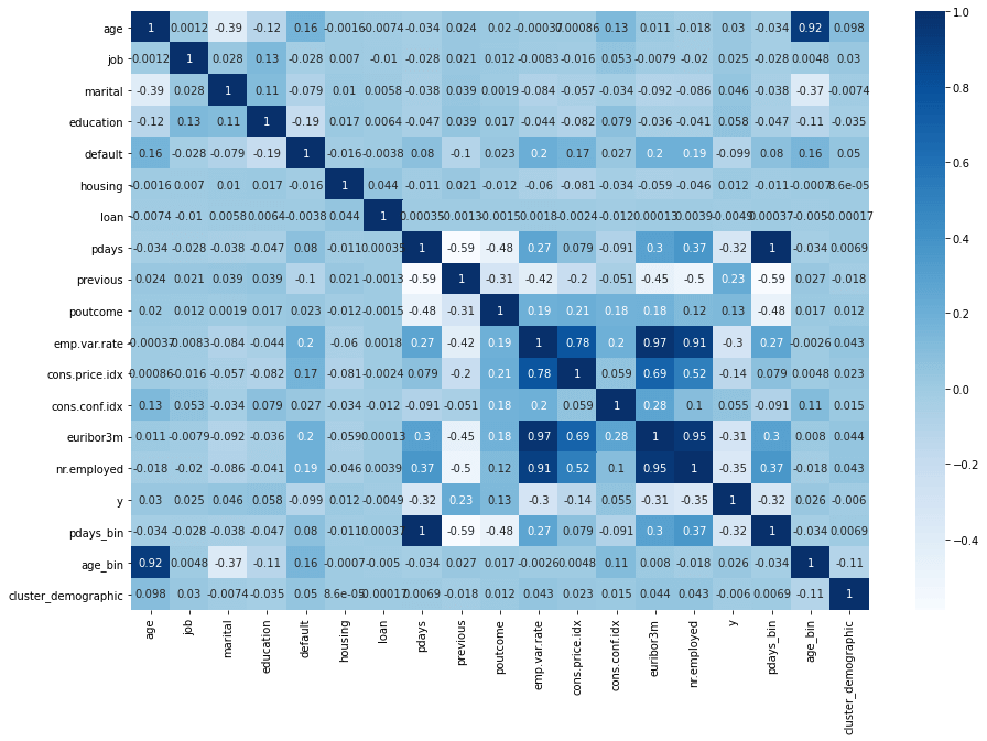
Creating a correlation heatmap is a good way to visualise potential collinearity. You can see from the colours below that age_bin and age are collinear, so are most of the economic indicator fields such as emp.var.rate, cons.price.idx, cons.conf.idx, euribor3m, and nr.employed. pdays and pdays_bin are perfectly collinear, so only one is needed. Similarly, pdays and previous have a strong negative correlation.
plt.figure(figsize=(15, 10))
sns.heatmap(df.corr(), annot=True, cmap="Blues")
There are quite a few different ways that we can identify which features we need to drop from the model (or group in a single feature) to improve the model’s performance. We could pair them up (i.e. euribor3m and cons.price.idx) and perform a permutation test and calculate the coefficient for each pair. We could also perform a chi-square test and check to see if the variables are independent. It’s also possible to do this through an automated approach using recursive feature elimination.
Recursive feature elimination
Recursive feature elimination or RFE fits a model to a data set in order to find and remove the weakest features. At each step it ranks features by coefficient or importance and removes one, helping to reduce collinearity. Too few features and the model returns poor results, while too many and performance quickly drops off. You can use any estimator model but DecisionTreeClassifier and RandomForestClassifier are most commonly used.
rfe = RFE(estimator=RandomForestClassifier(random_state=0), verbose=2)
rfe.fit(X, y)
Fitting estimator with 18 features.
Fitting estimator with 17 features.
Fitting estimator with 16 features.
Fitting estimator with 15 features.
Fitting estimator with 14 features.
Fitting estimator with 13 features.
Fitting estimator with 12 features.
Fitting estimator with 11 features.
Fitting estimator with 10 features.

RFE(estimator=RandomForestClassifier(random_state=0), verbose=2)
Printing out the n_features_ value returns the optimum number of features to use, while looping over the support_ and ranking_ values shows you which ones were supported and which weren’t. Putting these into a dataframe and sorting by the ranking gives a clearer view.
print("Optimum number of features: %d" % rfe.n_features_)
Optimum number of features: 9
df_features = pd.DataFrame(columns = ['feature', 'support', 'ranking'])

for i in range(X.shape[1]):
    row = {'feature': i,
           'support': rfe.support_[i],
           'ranking': rfe.ranking_[i]
          }
    df_features = df_features.append(row, ignore_index=True)

df_features.sort_values(by='ranking').head(20)
| feature | support | ranking | |
|---|---|---|---|
| 0 | 0 | True | 1 |
| 1 | 1 | True | 1 |
| 3 | 3 | True | 1 |
| 14 | 14 | True | 1 |
| 5 | 5 | True | 1 |
| 7 | 7 | True | 1 |
| 13 | 13 | True | 1 |
| 9 | 9 | True | 1 |
| 12 | 12 | True | 1 |
| 2 | 2 | False | 2 |
| 6 | 6 | False | 3 |
| 11 | 11 | False | 4 |
| 17 | 17 | False | 5 |
| 16 | 16 | False | 6 |
| 15 | 15 | False | 7 |
| 10 | 10 | False | 8 |
| 8 | 8 | False | 9 |
| 4 | 4 | False | 10 |
Finally, to select the features identified by RFE we can use the get_support() function. By passing in 1, this returns all supported features identified, to which we can pass to df.columns[] to return the columns and assign them to the new X dataframe, which now contains only our selected features.
selected_features = df.columns[rfe.get_support(1)]
selected_features
Index(['age', 'job', 'education', 'housing', 'pdays', 'poutcome',
       'cons.conf.idx', 'euribor3m', 'nr.employed'],
      dtype='object')
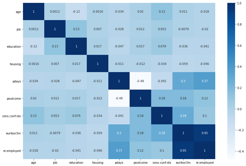
However, upon inspecting the correlation heatmap of the new X, it was clear that this didn’t work perfectly and two collinear features euribor3m and nr.employed were selected. To work around the issue with RFE including multicollinear features, I did some manually adjustments and played around with different feature combinations to see what worked best. The results were similar.
X = df[selected_features]

plt.figure(figsize=(15, 10))
sns.heatmap(X.corr(), annot=True, cmap="Blues")
Synthetic minority oversampling
Next, we need to deal with the class imbalance in this data set. As you’d imagine, there are many more lost sales than there are conversions. To help the model identify the relationships, we can use the Synthetic Minority Oversampling Technique or SMOTE. This introduces new data on the target variable to balance the classes.
y.value_counts()
0    36548
1     4640
Name: y, dtype: int64
smote = SMOTE()
X_smote, y_smote = smote.fit_sample(X, y)
y_smote.value_counts()
1    36548
0    36548
Name: y, dtype: int64
Split the train and test data
Now that the classes are balanced, we can split the data into the training and test datasets using train_test_split(). I’ve set a random_state to give reproducible results on the splits between runs and have assigned a third of the data to the test group.
X_train, X_test, y_train, y_test = train_test_split(X_smote,
                                                    y_smote,
                                                    test_size=0.33,
                                                    random_state=0)
Model selection
Next we need to identify the best model to use. To perform this step I have loaded up a range of packages for a wide range of different classification models, then I’ve created a dictionary containing the model name and the default model parameters.
import time
from xgboost import XGBClassifier
from lightgbm import LGBMClassifier
from sklearn.dummy import DummyClassifier
from sklearn.neighbors import KNeighborsClassifier
from sklearn.tree import DecisionTreeClassifier
from sklearn.ensemble import RandomForestClassifier
from sklearn.ensemble import AdaBoostClassifier
from sklearn.ensemble import GradientBoostingClassifier
from sklearn.naive_bayes import GaussianNB
from sklearn.model_selection import cross_val_score
from sklearn.metrics import classification_report
from sklearn.metrics import confusion_matrix
from sklearn.metrics import f1_score
from sklearn.metrics import accuracy_score
from sklearn.metrics import roc_auc_score
from sklearn.metrics import precision_score
from sklearn.metrics import recall_score
classifiers = {
    "DummyClassifier_stratified": DummyClassifier(strategy='stratified', random_state=0),
    "LGBMClassifier": LGBMClassifier(),
    "XGBClassifier": XGBClassifier(),
    "KNeighborsClassifier": KNeighborsClassifier(3),
    "DecisionTreeClassifier": DecisionTreeClassifier(),
    "RandomForestClassifier": RandomForestClassifier(),
    "AdaBoostClassifier": AdaBoostClassifier(),
    "GradientBoostingClassifier": GradientBoostingClassifier(),
    "GaussianNB": GaussianNB(),
}
Next we’ll loop through the classifiers, fit each one to the training data and then the results of cross fold validation using the ROC/AUC score to measure accuracy. The results for each round can be appended to the parent dataframe, so we can check and sort them to identify the top performer.
df_models = pd.DataFrame(columns=['model', 'run_time', 'roc_auc', 'roc_auc_std'])

for key in classifiers:

    print('*',key)

    start_time = time.time()

    classifier = classifiers[key]
    model = classifier.fit(X_train, y_train)

    cv = cross_val_score(model, X_train, y_train, cv=5, scoring='roc_auc')

    row = {'model': key,
           'run_time': format(round((time.time() - start_time)/60,2)),
           'roc_auc': cv.mean(),
           'roc_auc_std': cv.std(),
    }

    df_models = df_models.append(row, ignore_index=True)
* DummyClassifier_stratified
* LGBMClassifier
* XGBClassifier
* KNeighborsClassifier
* DecisionTreeClassifier
* RandomForestClassifier
* AdaBoostClassifier
* GradientBoostingClassifier
* GaussianNB
* XGBClassifier tuned
Examining the output from the model selection step shows that we achieved very good results. The XGBoost classifier performed particularly well.
df_models.sort_values(by='roc_auc', ascending=False).head(20)
| model | run_time | roc_auc | roc_auc_std | |
|---|---|---|---|---|
| 9 | XGBClassifier tuned | 0.11 | 0.972250 | 0.001138 |
| 2 | XGBClassifier | 0.06 | 0.971588 | 0.000940 |
| 1 | LGBMClassifier | 0.02 | 0.965668 | 0.001494 |
| 5 | RandomForestClassifier | 0.43 | 0.965424 | 0.001565 |
| 7 | GradientBoostingClassifier | 0.32 | 0.915796 | 0.001523 |
| 4 | DecisionTreeClassifier | 0.02 | 0.900602 | 0.002601 |
| 3 | KNeighborsClassifier | 0.07 | 0.888723 | 0.003280 |
| 6 | AdaBoostClassifier | 0.1 | 0.845891 | 0.001610 |
| 8 | GaussianNB | 0.0 | 0.749527 | 0.002500 |
| 0 | DummyClassifier_stratified | 0.0 | 0.497062 | 0.005256 |
Assessing performance
When it comes to assessing models, there’s more to it than simply picking the one with the best score, especially when it comes to accuracy. It’s where the model that goes wrong that often matters. To better explain, let’s take a look at the four possible outcomes:
- True positive - The model correctly predicted that a customer would purchase
- True negative - The model correctly predicted that a customer wouldn’t purchase
- False positive - The model incorrectly predicted that a customer would purchase
- False negative - The model incorrectly predicted that a customer wouldn’t purchase
Clearly, more true positives is a good thing, as it brings in more orders. Similarly, more true negatives is good, because sales staff waste less time by contacting unresponsive customers. However, there are trade-offs when it comes to false positives and false negatives. Too many false positives will waste the time of the sales team, while too many false negatives will mean the model isn’t predicting potential sales.
classifiers = {
    "XGBClassifier": XGBClassifier(),
    "LGBMClassifier": LGBMClassifier(),
    "RandomForestClassifier": RandomForestClassifier(),
}

df_models = pd.DataFrame(columns=['model', 'tp', 'tn', 'fp', 'fn', 'correct', 'incorrect',
                                  'accuracy', 'precision', 'recall', 'f1', 'roc_auc'])

for key in classifiers:

    classifier = classifiers[key]
    model = classifier.fit(X_train, y_train)
    y_pred = model.predict(X_test)

    tn, fp, fn, tp = confusion_matrix(y_test, y_pred).ravel()
    accuracy = accuracy_score(y_test, y_pred)
    precision = precision_score(y_test, y_pred)
    recall = recall_score(y_test, y_pred)
    f1 = f1_score(y_test, y_pred)
    roc_auc = roc_auc_score(y_test, y_pred)

    row = {'model': key,
           'tp': tp,
           'tn': tn,
           'fp': fp,
           'fn': fn,
           'correct': tp+tn,
           'incorrect': fp+fn,
           'accuracy': round(accuracy,3),
           'precision': round(precision,3),
           'recall': round(recall,3),
           'f1': round(f1,3),
           'roc_auc': round(roc_auc,3),
    }

    df_models = df_models.append(row, ignore_index=True)
I’ve skipped the introduction of StandardScaler above, but I’d advise trying this to see if it improves your model performance.
df_models.sort_values(by='roc_auc', ascending=False).head(20)
| model | tp | tn | fp | fn | correct | incorrect | accuracy | precision | recall | f1 | roc_auc | |
|---|---|---|---|---|---|---|---|---|---|---|---|---|
| 0 | XGBClassifier | 11045 | 11390 | 576 | 1111 | 22435 | 1687 | 0.930 | 0.950 | 0.909 | 0.929 | 0.930 |
| 2 | RandomForestClassifier | 11060 | 11075 | 891 | 1096 | 22135 | 1987 | 0.918 | 0.925 | 0.910 | 0.918 | 0.918 |
| 1 | LGBMClassifier | 10956 | 11136 | 830 | 1200 | 22092 | 2030 | 0.916 | 0.930 | 0.901 | 0.915 | 0.916 |
Hyperparameter tuning
Finally, we can select the XGBClassifier() as our chosen model and apply hyperparameter tuning to see if we can gain any further improvements. We’ll use GridSearchCV() to do this. This involves creating a series of list of values to test and then passing them into GridSearchCV via a param_grid. After checking all the iterations, the grid search will return the optimum model parameters to use and the maximum score achieved.
n_estimators = [50]
learning_rate = [0.1]
max_depth = [5, 10, 20]
min_child_weight = [1, 2]
scale_pos_weight = [1, 2]
gamma = [0.9, 1.0]
subsample = [0.9]
colsample_bytree = [0.8, 1.0]

param_grid = dict(
                n_estimators=n_estimators,
                learning_rate=learning_rate,
                max_depth=max_depth,
                min_child_weight=min_child_weight,
                scale_pos_weight=scale_pos_weight,
                gamma=gamma,
                subsample=subsample,
                colsample_bytree=colsample_bytree,
)

model = XGBClassifier(random_state=0)

grid_search = GridSearchCV(estimator=model,
                           param_grid=param_grid,
                           scoring='roc_auc',
                           )

best_model = grid_search.fit(X_train, y_train)
best_score = round(best_model.score(X_test, y_test), 4)
best_params = best_model.best_params_

print('Best score:', best_score)
print('Optimum parameters:', best_params)
Best score: 0.9724

Optimum parameters: {'colsample_bytree': 0.8, 'gamma': 1.0, 'learning_rate': 0.1,
'max_depth': 20, 'min_child_weight': 1, 'n_estimators': 50, 'scale_pos_weight': 1,
'subsample': 0.9}
Final check
As a final check, we’ll re-run the tuned model and compare the score against the other models using cross validation. We get a tiny bit more improvement, with the final ROC/AUC ending up at 0.972250. We’re able to predict which customers will convert with very strong accuracy.
classifiers = {
    "DummyClassifier_stratified": DummyClassifier(strategy='stratified', random_state=0),
    "LGBMClassifier": LGBMClassifier(),
    "XGBClassifier": XGBClassifier(),
    "KNeighborsClassifier": KNeighborsClassifier(3),
    "DecisionTreeClassifier": DecisionTreeClassifier(),
    "RandomForestClassifier": RandomForestClassifier(),
    "AdaBoostClassifier": AdaBoostClassifier(),
    "GradientBoostingClassifier": GradientBoostingClassifier(),
    "GaussianNB": GaussianNB(),
    "XGBClassifier tuned": XGBClassifier(random_state=0,
                      colsample_bytree = 0.8,
                      gamma = 1.0,
                      learning_rate = 0.1,
                      max_depth = 20,
                      min_child_weight = 1,
                      n_estimators = 50,
                      scale_pos_weight = 1,
                      subsample = 0.9
                     ),
}
df_models = pd.DataFrame(columns=['model', 'run_time', 'roc_auc', 'roc_auc_std'])

for key in classifiers:

    print('*',key)

    start_time = time.time()

    classifier = classifiers[key]
    model = classifier.fit(X_train, y_train)

    cv = cross_val_score(model, X_train, y_train, cv=5, scoring='roc_auc')

    row = {'model': key,
           'run_time': format(round((time.time() - start_time)/60,2)),
           'roc_auc': cv.mean(),
           'roc_auc_std': cv.std(),
    }

    df_models = df_models.append(row, ignore_index=True)
* DummyClassifier_stratified
* LGBMClassifier
* XGBClassifier
* KNeighborsClassifier
* DecisionTreeClassifier
* RandomForestClassifier
* AdaBoostClassifier
* GradientBoostingClassifier
* GaussianNB
* XGBClassifier tuned
df_models.sort_values(by='roc_auc', ascending=False).head(20)
| model | run_time | roc_auc | roc_auc_std | |
|---|---|---|---|---|
| 9 | XGBClassifier tuned | 0.1 | 0.972250 | 0.001138 |
| 2 | XGBClassifier | 0.06 | 0.971588 | 0.000940 |
| 1 | LGBMClassifier | 0.02 | 0.965668 | 0.001494 |
| 5 | RandomForestClassifier | 0.43 | 0.965402 | 0.001627 |
| 7 | GradientBoostingClassifier | 0.32 | 0.915793 | 0.001521 |
| 4 | DecisionTreeClassifier | 0.02 | 0.900045 | 0.002561 |
| 3 | KNeighborsClassifier | 0.06 | 0.888723 | 0.003280 |
| 6 | AdaBoostClassifier | 0.1 | 0.845891 | 0.001610 |
| 8 | GaussianNB | 0.0 | 0.749527 | 0.002500 |
| 0 | DummyClassifier_stratified | 0.0 | 0.497062 | 0.005256 |
Matt Clarke, Saturday, March 06, 2021


Other posts you might like

How to tune a LightGBMClassifier model with Optuna
The LightGBM model is a gradient boosting framework that uses tree-based learning algorithms, much like the popular XGBoost model. LightGBM supports both classification and regression tasks, and is known for...

How to create a customer retention model with XGBoost
Although all business know the importance of retaining customers, few companies are actually able to measure customer retention accurately, and fewer still can predict which ones will churn or be...
