How to analyse Average Order Value with Jenks natural breaks classification
Learn how to analyse Average Order Value using the Google Analytics API and Jenks natural breaks classification to reveal hidden patterns in your data and identify ways to boost your AOV.

Average Order Value or AOV is one of the most critical ecommerce metrics. Along with your sessions and conversion rate, it ultimately controls how much revenue an ecommerce business generates. However, averages lie and conceal hidden data, so failing to examine what lies beneath an ecommerce site’s AOV metric is a missed opportunity to find ways to grow your ecommerce sales.
In this project, I’ll show you how to analyse the Average Order Value of your ecommerce business using the Google Analytics API and GAPandas, visualise the distribution of order values with Seaborn, and identify the natural clusters in order values using a classification technique called Jenks natural breaks classification. I’ll also explain how you can use the data to help increase your site’s AOV.
What is Jenks natural breaks classification?
Jenks natural breaks classification, also known as the Jenks optimisation method, or Fisher Jenks natural splits, is a data clustering technique designed to place values into naturally occurring classes or groups via binning or bucketing data.
It’s closely related to Fisher’s Discriminant Analysis and Otsu’s Method and works by aiming to minimise the average deviation from the class mean, while maximising each class’s deviation from the means of other classes, thus creating easily identifiable groups.
Thankfully, you don’t need to understand the exact maths used in the algorithm in order to apply it to your data since the Python package jenkspy implements it to allow you to create a specified number of classes, a bit like k-means clustering. It is a useful technique for clustering data - I’ve used it here for analysing Average Order Values, but I’ve also applied it to the creation of segments in RFM models.
Install the packages
First, open a Jupyter notebook and install the jenkspy and gapandas packages by entering the commands below and then executing the cell. The jenkspy package will be used to create the Jenks natural breaks classification, while the GAPandas package will be used to extract ecommerce data directly from your Google Analytics account using the API. If you have access to transactional data from another source, you can skip ahead.
!pip3 install gapandas
!pip3 install jenkspy
Load the packages
Once the packages are installed, enter the below commands to import the packages. The code cells below the import statements are used to control the appearance of some Seaborn data visualisations we’ll be creating in later steps.
import pandas as pd
import gapandas as gp
import seaborn as sns
import jenkspy
%config InlineBackend.figure_format = 'retina'
sns.set_context('notebook')
sns.set(rc={'figure.figsize':(15, 6)})
Configure your Google Analytics API connection
Next, you’ll need to configure your Google Analytics API connection. GAPandas requires you to create a client secrets JSON keyfile to authenticate against your Google Analytics data. These can be created via the Google API Console in just a couple of minutes. You’ll also need the view ID for the Google Analytics property to you want to query. Once you’ve got these, pass the key file path to get_service() to return the service object and assign your GA view ID to a variable.
service = gp.get_service('client_secrets.json', verbose=False)
view = '123456789'
Query the Google Analytics API with GAPandas
With a working connection to Google Analytics in place, we can create a little function to fetch some order data from the Google Analytics API using GAPandas. This takes the service and view variables created above, plus the start_date and end_date. Optionally, you can also pass in a Google Analytics filter to allow you to compare order data from different marketing channels, for example.
def orders(service,
           view,
           start='2021-01-01',
           end='2021-01-01',
           filters=None):
    """Return order data.

    Args:
        service (object): Google Analytics service connection.
        view (string): Google Analytics view ID, i.e. 123456789
        start (string, optional): Optional start date YYYY-MM-DD.
        end (string, optional): Optional end date YYYY-MM-DD.
        filters (string, optional): Optional filters

    Returns:
        object: Pandas dataframe.
    """

    payload = {
        'start_date': start,
        'end_date': end,
        'metrics': 'ga:transactionRevenue',
        'dimensions': 'ga:transactionId',
        'filters': filters,
    }

    df = gp.run_query(service, view, payload)
    return df
With your function setup, pass in the required values and assign the output to a Pandas dataframe called df. This will return the transactionId value and the transactionRevenue value from your Google Analytics data for the period selected and put the data into a neatly formatted Pandas dataframe.
df = orders(service, view)
df.head()
| transactionId | transactionRevenue | |
|---|---|---|
| 0 | 001000002 | 74.99 |
| 1 | 001000003 | 79.99 |
| 2 | 0AQ752732 | 45.99 |
| 3 | 0BY752758 | 15.70 |
| 4 | 0LQ752349 | 51.28 |
Calculate the Average Order Value
To get a handle on the Average Order Value for this site, we can calculate the AOV using the Pandas mean() function. Appending .mean() to the df['transactionRevenue'] will return the AOV for the selected period, which is £65.75. If you calculate the min() and max() values for the column you’ll see that AOVs range from £3.49 and rise to £2099.62, so that £65.75 figure is really obscuring lots of potentially useful information about customer order values.
df['transactionRevenue'].mean()
65.7515950792327
df['transactionRevenue'].min()
3.49
df['transactionRevenue'].max()
2099.62
Visualise the distribution of order values
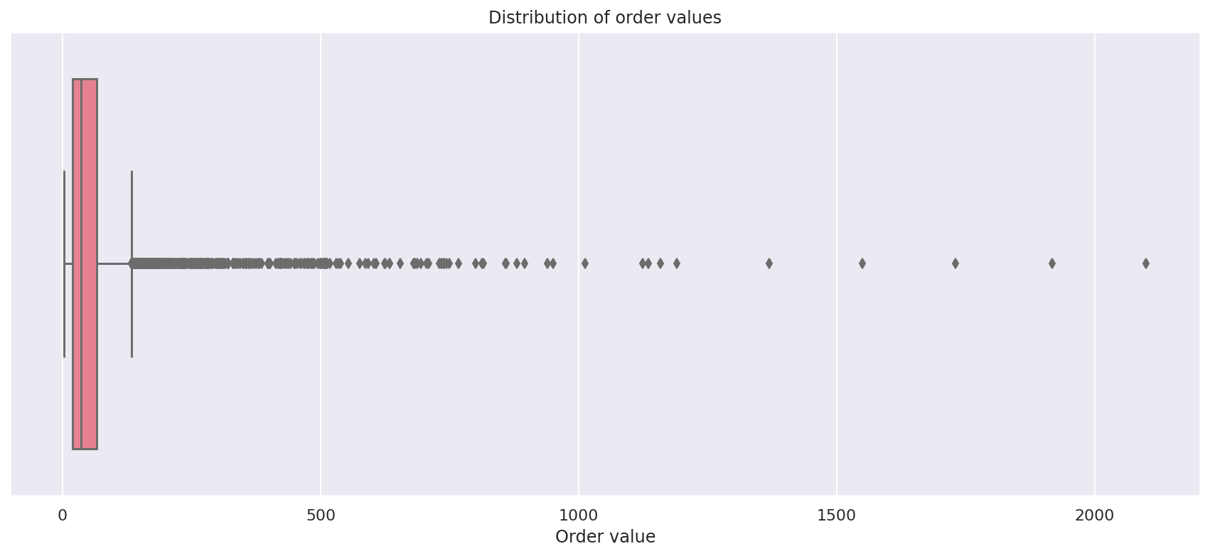
To get a better understanding of the distribution of values in the transactionRevenue column we can use Seaborn for some data visualisation. First, we’ll create a Seaborn boxplot or box-and-whisker diagram.
A boxplot is used to visualise the distribution of quantitative data and splits it into quartiles and clearly shows outliers positioned above the upper whisker. For our data, you can clearly see that the majority of orders fall in the lower bounds, with lots of outliers caused by higher value orders being placed.
plot = sns.boxplot(x=df["transactionRevenue"], palette="husl")
plot.set_title('Distribution of order values')
plot.set_xlabel('Order value')
Text(0.5, 0, 'Order value')
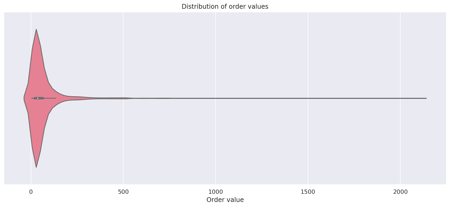
The violin plot is another way to observe the distribution of data. It works a bit like a boxplot, but rather than show a box with quartile markers, the width of the violin plot is denoted by the number of values present.
plot = sns.violinplot(x=df["transactionRevenue"], palette="husl")
plot.set_title('Distribution of order values')
plot.set_xlabel('Order value')
Text(0.5, 0, 'Order value')
Create a Jenks breaks classification
Now we’ve got an understanding of the data through those Seaborn visualisations, we can move on to creating the Jenks breaks classification. To do this you simply pass the Pandas dataframe column to the jenks_breaks() function of jenkspy along with the number of classes you wish to create. I’ve selected five, purely for practical demonstration purposes, but I’d recommend fiddling with these until you get the right outputs for your ecommerce business.
jenks_breaks = jenkspy.jenks_breaks(df['transactionRevenue'], nb_class=5)
If you print the output from the Jenks breaks classification, you’ll get back a list of values representing the bounds for each break or natural split identified.
jenks_breaks
[3.49, 70.5, 199.09, 450.88, 1012.45, 2099.62]
Next we’ll use the values from jenks_breaks to identify the upper and lower bound for order values within each of the AOV classes the Jenks natural splits classification has identified. We’ll assign these labels as strings and put them back into the dataframe.
jenks_labels = [
    '£' + str(jenks_breaks[0]) + ' to £' + str(jenks_breaks[1]),
    '£' + str(jenks_breaks[1]) + ' to £' + str(jenks_breaks[2]),
    '£' + str(jenks_breaks[2]) + ' to £' + str(jenks_breaks[3]),
    '£' + str(jenks_breaks[3]) + ' to £' + str(jenks_breaks[4]),
    '£' + str(jenks_breaks[4]) + ' to £' + str(jenks_breaks[5]),
]

df['jenks_break'] = pd.cut(df['transactionRevenue'], bins=jenks_breaks, labels=jenks_labels)
df.head()
| transactionId | transactionRevenue | jenks_break | |
|---|---|---|---|
| 0 | 001000002 | 74.99 | £70.5 to £199.09 |
| 1 | 001000003 | 79.99 | £70.5 to £199.09 |
| 2 | 0AQ752732 | 45.99 | £3.49 to £70.5 |
| 3 | 0BY752758 | 15.70 | £3.49 to £70.5 |
| 4 | 0LQ752349 | 51.28 | £3.49 to £70.5 |
Now each transaction has been labelled with the class generated by the Jenks natural breaks classification we can create another Pandas dataframe to summarise the data. To do this we’ll group by the jenks_break column label and use agg() to aggregate the data and calculate the number of orders, total revenue, minimum order value, maximum order value, and mean order value (or AOV) at each of the Jenks breaks. We’ll also calculate the percentage of orders and revenue generated by each break.
df_breaks = df.groupby('jenks_break').agg(
    orders=('transactionId', 'count'),
    revenue=('transactionRevenue', sum),
    min_order_value=('transactionRevenue', min),
    max_order_value=('transactionRevenue', max),
    mean_order_value=('transactionRevenue', 'mean'),
).sort_values(by='mean_order_value', ascending=True).reset_index().round(2).head(5)

df_breaks['pc_orders'] = round((df_breaks['orders'] / df_breaks['orders'].sum()) * 100, 1)
df_breaks['pc_revenue'] = round((df_breaks['revenue'] / df_breaks['revenue'].sum()) * 100, 1)
Although the AOV we identified in this dataset was £65.75, you can see that there is actually a massive variation in the data. The largest AOV band is made up of the smallest order values, with orders between £3.49 and £70.50 generating 77% of the order volume and 36% of the revenue, with an AOV of £31.02 in this band. That means that orders with an above average AOV generate just 23% or so of the total orders, but contribute 64% of the revenue.
df_breaks
| jenks_break | orders | revenue | min_order_value | max_order_value | mean_order_value | pc_orders | pc_revenue | |
|---|---|---|---|---|---|---|---|---|
| 0 | £3.49 to £70.5 | 3707 | 115007.04 | 3.60 | 70.50 | 31.02 | 77.3 | 36.5 |
| 1 | £70.5 to £199.09 | 824 | 91019.41 | 70.87 | 199.09 | 110.46 | 17.2 | 28.9 |
| 2 | £199.09 to £450.88 | 185 | 53374.67 | 200.13 | 450.88 | 288.51 | 3.9 | 16.9 |
| 3 | £450.88 to £1012.45 | 69 | 42662.97 | 455.25 | 1012.45 | 618.30 | 1.4 | 13.5 |
| 4 | £1012.45 to £2099.62 | 9 | 13273.58 | 1124.67 | 2099.62 | 1474.84 | 0.2 | 4.2 |
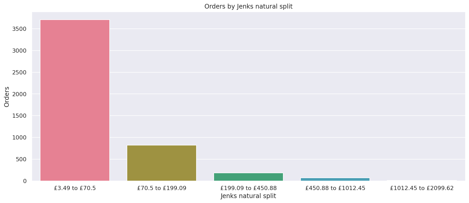
Visualise the orders in each break
To get a better impression of the contribution generated by each Jenks natural split class we can use a Seaborn barplot. To create these we need to pass in the df_breaks dataframe above to the data argument of sns.barplot() and set the x value to the jenks_breaks column and the y value to the orders data. This clearly shows that the bulk of orders are small and lower in value.
plot = sns.barplot(x="jenks_break", y="orders", data=df_breaks, estimator=sum, palette="husl")
plot.set_title('Orders by Jenks natural split')
plot.set_ylabel('Orders')
plot.set_xlabel('Jenks natural split')
Text(0.5, 0, 'Jenks natural split')
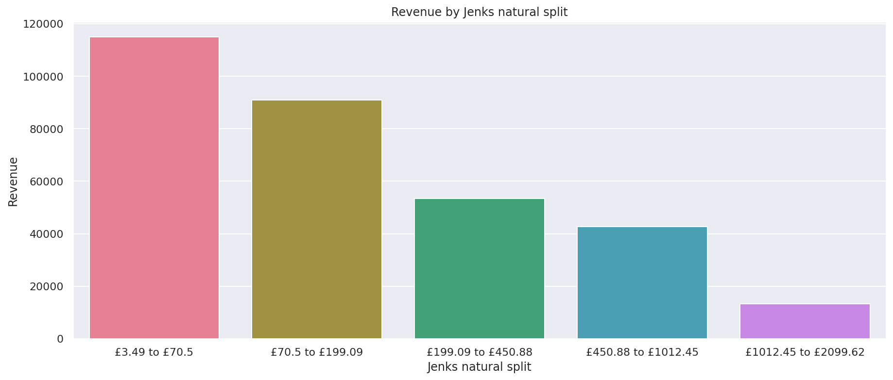
Visualise the revenue generated from each break
Finally, we can repeat the process by pass in the revenue column to see how revenue contribution is distributed across the Jenks natural split classes. Those low value orders contribute the most as far as individual classes are concerned, but the higher value breaks contribute significantly more revenue overall.
plot = sns.barplot(x="jenks_break", y="revenue", data=df_breaks, estimator=sum, palette="husl")
plot.set_title('Revenue by Jenks natural split')
plot.set_ylabel('Revenue')
plot.set_xlabel('Jenks natural split')
Text(0.5, 0, 'Jenks natural split')
How can I use these data?
There are two really useful applications for Jenks natural splits classifications of AOV in ecommerce, but they’re both very similar.
Setting free delivery thresholds
The first application of Fisher Jenks natural breaks or Jenks natural splits is to guide an ecommerce business on where they should position their free delivery threshold. Most ecommerce websites give customers free delivery when they spend over a certain amount, as this can encourage customers to spend slightly more than they intended in order to save a few pounds on the delivery charge.
By using Jenks natural splits you can identify where those delivery thresholds should be positioned. For example, in the data above, I’d propose testing a free delivery threshold around the £70 mark to encourage customers in the first break to stretch and spend a little more.
Similarly, you could add a free delivery threshold for a premium delivery service for the higher breaks. For example, spend over £200 and get free next day delivery. You’ll probably want to increase the number of classes in your model before you do this to ensure you truly understand the distribution in order values.
Setting promotion thresholds
Similarly, the other application of Jenks natural splits classification of order values is in setting coupon promotion thresholds. For example, “Spend over £100 and get £5 off”, or “Spend over £200 and get £15 off”.
These should work in exactly the same way, and you should position your tiered discount just in front of the average value for the break or the upper boundary of the break (you’ll need to test this to find what works best for you).
The two approaches will not only help you understand your customer data better, but they’ll also provide a practical means for you to assist your ecommerce team in driving the AOV upwards, generating both more profit and more margin.
Matt Clarke, Friday, February 04, 2022


Other posts you might like

How to use the Pandas truncate() function
Have you ever needed to chop the top or bottom off a Pandas dataframe, or extract a specific section from the middle? If so, there’s a Pandas function called truncate()...

How to use Spacy for noun phrase extraction
Noun phrase extraction is a Natural Language Processing technique that can be used to identify and extract noun phrases from text. Noun phrases are phrases that function grammatically as nouns...
