How to analyse product consumption and repurchase rates
Learn how to shape your product, content, and pricing strategy by analysing product consumption and repurchase rates by product using Pandas.

You can learn many things about your products from the purchase behaviours and product consumption and product replenishment of your customers. Some items are purchased individually, some items are purchased in small groups, and others are bought in bulk.
Some products are only ever purchased once by each customer, while others are trialled, and the customer either repurchases, trials an alternative, or goes somewhere else. Knowing these things can help you in several ways and can help several departments within the typical ecommerce business improve their KPIs and generate more profit for the business.
In this project, we’re going to take a look some different ways of measuring product consumption and product repurchase rates to identify potential strategic changes that could be made. To do this we first need to understand product consumption and repurchase rates.
Product consumption
Product consumption is a measure of the typical volumes of each product that get purchased. Certain items are usually only purchased individually, either because they’re expensive, or because customers don’t need more than one unit.
For example, most people only ever buy a single fridge, phone, or ladder. Offering bulk discounts on multiple units probably won’t sell you any more units, unless you’re a B2B retailer.
However, others are commonly purchased as multiple units in a single basket, or purchased in bulk. How many people buy a single banana or potato, for example? Customers expect such products to be bundled in larger quantities (imagine the inconvenience of purchasing individual blueberries, for example), and would likely want a discount for purchasing a higher volume.
Product consumption is typically measured in ecommerce using a metric such as “average items per basket”. Since this metric is directly correlated with average order value, ecommerce merchandisers and marketers will be aiming to influence customers to buy slightly more and make both metrics go up.
Factors affecting product consumption
| Product type | Will a customer ever need several of this product type? What is the typical purchase quantity for the product type? |
| Customer need | How many items does the customer actually need? Is the pack size appropriate to the customer's requirements? |
| Product price | Is the product price high or low? High ticket price items are rarely sold in larger quantities. |
| Product perishability | Can the item be purchased in bulk and kept for later use? Does it perish and require replacement periodically? |
| Product availability | Can customers buy as much as they need? Does the retailer often run out of stock? |
| Product promotions | Could a promotion be used to encourage customers to purchase more than they require? |
| Despatch speed | Does it take a long time to deliver? Might customers stockpile to avoid running out? |
| Panic buying | Are customers panic buying? Will they run out of toilet roll, alcohol hand gel, or cat food? |
 Most people stockpile toilet roll (especially in pandemics). Picture by “Hello I’m Nik”, Unsplash.
Repurchase rates
The repurchase rate, or repurchase index, is calculated by identifying the number of customers who re-purchased a given product over the total number of customers who purchased the product, sometimes over a specific time period. It aims to measure the proportion of customers who purchased a product once, then purchased the same item again.
By introducing a time element, such as the repurchase rate for a rolling 12 month window, you can measure changes in product purchasing behaviour. Perhaps you increased your price and customers switched to cheaper brands or started shopping elsewhere? Or, maybe you’ve changed your product recommendations or run a promotion that has encouraged customers to buy an item again.
As with the average items per basket metric, merchandisers and marketers want customers to repurchase products. This helps strengthen the customer relationship, which in turn increases the likelihood of customer retention and increases CLV and customer equity. Of course, with so many factors influencing the likelihood to repurchase, it’s not all within the hands of the ecommerce and marketing team, but much is.
If repurchase rates on SKUs are high, adding a subscription option may be advantageous. However, it could be a waste of development resource if few products ever get purchased for replenishment.
Factors affecting repurchase rate
| Product type | Is the product a consumable? Will it require replenishment or replacement, or is it a one-off purchase? |
| Product lifespan | How long will the item last the customer? Longer lasting items may be replaced with alternatives if the product originally purchased is no longer sold. |
| Pack size | If the product is a consumable, how long will the pack size they purchased last them? |
| Product satisfaction | Did the customer like the product enough to purchase it again? Will they trial an alternative product to find one that suits their needs, or just go elsewhere? |
| Product price | Has the price gone up since the customer last purchased it? Did they think it was good value? |
| Customer experience | Was the customer experience good? Did the right item arrive on time and in good condition? If something went wrong, did the company utilise service recovery? |
| Product availability | Was the product available again if the customer did want to repurchase it? Was it in stock at the time of their visit? Had it been discontinued? |
| Despatch speed | Can the retailer get the product to the customer in time to meet their demand, or will they look for an alternative or shop elsewhere? |
| Findability | Can the customer find the item they ordered before to repurchase it? |
 Picture by Charisse Kenion, Unsplash.
Load the packages
The vast majority of our work here can be done within Pandas, but we’ll also need a bit of NumPy, and some Seaborn and Matplotlib for data visualisation. Open a Jupyter notebook and load the required packages.
import pandas as pd
import numpy as np
import seaborn as sns
import matplotlib.pyplot as plt
Optionally, if you want to generate sharper, more stylish charts, you can pass in some additional commands to Seaborn to set up themes and retina mode visualisations.
%config InlineBackend.figure_format = 'retina'
sns.set_context('notebook')
sns.set(rc={'figure.figsize':(15, 6)})
sns.set_style("dark")
sns.set()
Load the data
Next, load up a transactional item dataset. This needs to include the SKU (stock keeping unit or product code), the quantity of units purchased, the unit price paid, the customer ID, the order ID, and the order date.
df = pd.read_csv('transaction_items.csv')
df.sample(5)
| order_id | sku | quantity | unit_price | customer_id | order_date | |
|---|---|---|---|---|---|---|
| 543793 | 516619 | 1205723 | 1 | 18.99 | 306400.0 | 2020-05-06 13:38:19 |
| 486226 | 494435 | 2855306 | 1 | 99.00 | 391147.0 | 2020-04-09 09:37:18 |
| 234270 | 394059 | 1690165 | 1 | 10.62 | 296269.0 | 2019-02-15 10:48:59 |
| 618417 | 545221 | 931539 | 1 | 4.19 | 400233.0 | 2020-06-13 18:51:15 |
| 137526 | 354267 | 1272246 | 2 | 11.99 | 231294.0 | 2018-06-02 18:39:52 |
Create a repurchase rate function
While you can calculate each metric individually in Jupyter and examine the output if you wish, it’s helpful to create a reusable function for this analysis so you can re-run it again in the future.
The aim of our function will be to segment the product portfolio based on product consumption and repurchase behaviour, so we can identify which items are commonly purchased individually versus those purchased in multiples, and identify which products are purchased once by a customer, versus those that are purchased multiple times.
This uses a bit of data wrangling to calculate the purchase consumption metrics for each SKU in the transactional item dataset, and then calculates the number of times each SKU was purchased individually in orders, and purchased once by customers.
It then uses those data to calculate the “bulk purchase rate” (indicating the percentage of orders that include the same SKU multiple times) and the “repurchase rate” (which shows the percentage of customers who purchased the same SKU again in a future order).
def get_repurchase_rates(df):
    """Given a Pandas DataFrame of transactional items, this function returns
    a Pandas DataFrame containing the purchase behaviour and repurchase
    behaviour for each SKU.

    Parameters
    ----------

    df: Pandas DataFrame
        Required columns: sku, order_id, customer_id, quantity, unit_price

    Returns
    -------
    df: Pandas DataFrame
        sku, order_id, customer_id, quantity, unit_price, avg_unit_price, avg_line_price, revenue,
        times_purchased, purchased_individually, purchased_once, items, orders, customers,
        bulk_purchases, bulk_purchase_rate, repurchases, repurchase_rate

    """

    # Count the number of times each customer purchased each SKU
    df['times_purchased'] = df.groupby(['sku','customer_id'])['order_id'].transform('count')

    # Count the number of times the SKU was purchased individually within orders
    df['purchased_individually'] = df[df['quantity']==1].\
        groupby('sku')['order_id'].transform('count')
    df['purchased_individually'] = df['purchased_individually'].fillna(0)

    # Count the number of times the SKU was purchased once only by customers
    df['purchased_once'] = df[df['times_purchased']==1].\
        groupby('sku')['order_id'].transform('count')
    df['purchased_once'] = df['purchased_once'].fillna(0)

    # Calculate line price
    df['line_price'] = df['unit_price'] * df['quantity']

    # Get unique SKUs and count total items, orders, and customers
    df_skus = df.groupby('sku').agg(
        revenue=('line_price', 'sum'),
        items=('quantity', 'sum'),
        orders=('order_id', 'nunique'),
        customers=('customer_id', 'nunique'),
        avg_unit_price=('unit_price', 'mean'),
        avg_line_price=('line_price', 'mean')
    )

    # Calculate the average number of units per order
    df_skus = df_skus.assign(avg_items_per_order=( df_skus['items'] / df_skus['orders'] ))

    # Calculate the average number of items per customer
    df_skus = df_skus.assign(avg_items_per_customer=( df_skus['items'] / df_skus['customers'] ))

    # Merge the dataframes
    df_subset = df[['sku','purchased_individually','purchased_once']].fillna(0)
    df_subset.drop_duplicates('sku', keep='first', inplace=True)
    df_skus = df_skus.merge(df_subset, on='sku', how='left')

    # Calculate bulk purchase rates
    df_skus = df_skus.assign(bulk_purchases = (df_skus['orders'] -\
                                               df_skus['purchased_individually']) )
    df_skus = df_skus.assign(bulk_purchase_rate = (df_skus['bulk_purchases'] \
                                                   / df_skus['orders']) )

    # Calculate repurchase rates
    df_skus = df_skus.assign(repurchases = (df_skus['orders'] - df_skus['purchased_once']) )
    df_skus = df_skus.assign(repurchase_rate = (df_skus['repurchases'] / df_skus['orders']) )

    return df_skus
Next, we can run the get_repurchase_rates() function above on our transactional items dataframe to return a new dataframe containing the product consumption and repurchase metrics for each SKU in the product portfolio. Using T to transpose the data makes it a bit easier to fit on the screen.
df = get_repurchase_rates(df)
df.sample(3).T
| 3411 | 4114 | 4222 | |
|---|---|---|---|
| sku | 2.384919e+06 | 2.855088e+06 | 2.855197e+06 |
| revenue | 1.466810e+03 | 1.943150e+03 | 3.749750e+03 |
| items | 8.400000e+01 | 2.500000e+01 | 5.250000e+02 |
| orders | 8.100000e+01 | 2.100000e+01 | 4.790000e+02 |
| customers | 7.900000e+01 | 2.100000e+01 | 4.590000e+02 |
| avg_unit_price | 1.746185e+01 | 7.769476e+01 | 7.359812e+00 |
| avg_line_price | 1.810877e+01 | 9.253095e+01 | 7.828288e+00 |
| avg_items_per_order | 1.037037e+00 | 1.190476e+00 | 1.096033e+00 |
| avg_items_per_customer | 1.063291e+00 | 1.190476e+00 | 1.143791e+00 |
| purchased_individually | 7.800000e+01 | 0.000000e+00 | 4.420000e+02 |
| purchased_once | 7.700000e+01 | 2.100000e+01 | 4.410000e+02 |
| bulk_purchases | 3.000000e+00 | 2.100000e+01 | 3.700000e+01 |
| bulk_purchase_rate | 3.703704e-02 | 1.000000e+00 | 7.724426e-02 |
| repurchases | 4.000000e+00 | 0.000000e+00 | 3.800000e+01 |
| repurchase_rate | 4.938272e-02 | 0.000000e+00 | 7.933194e-02 |
Binning repurchase rate data
The raw values are useful but labeling the data will make it much easier to understand. For this we can use the quantile-based discretization approach to bin or bucket data and assign labels to each product based on the repurchase rate or bulk purchasing rate.
The Pandas cut() function makes this quite simple. We’ll use this to assign the repurchase_rate metric to five bins that we will label according to the rate. There’s no need to set the bounds for the bins here, as the function can do this for us.
def get_repurchase_rate_label(df):

    labels = ['Very low repurchase',
              'Low repurchase',
              'Moderate repurchase',
              'High repurchase',
              'Very high repurchase']
    df['repurchase_rate_label'] = pd.cut(df['repurchase_rate'],
                                          bins=5,
                                          labels=labels)
    return df
df = get_repurchase_rate_label(df)
df['repurchase_rate_label'].value_counts()
Very low repurchase     4344
Low repurchase           975
Very high repurchase     646
Moderate repurchase      200
High repurchase           29
Name: repurchase_rate_label, dtype: int64
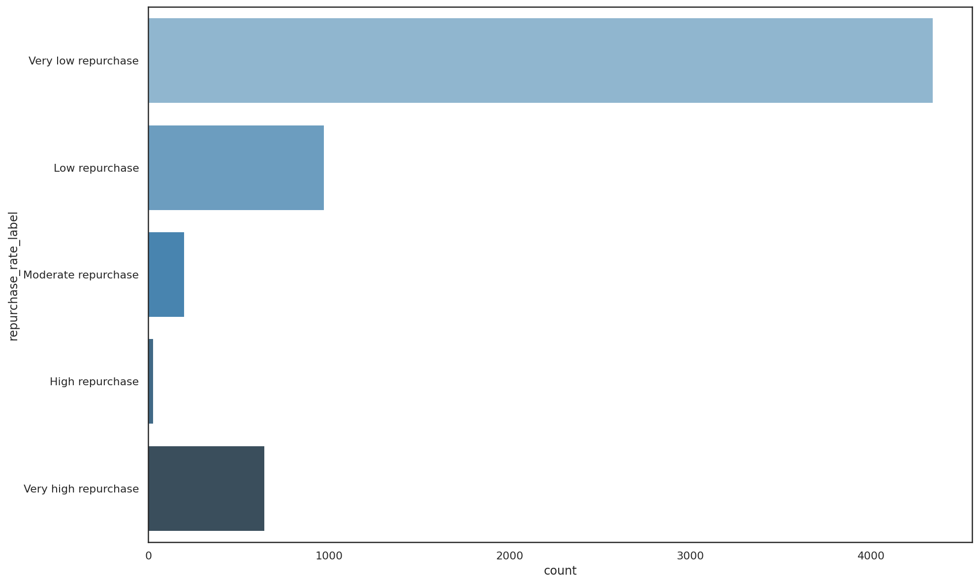
Running the function on our data and examining the number of SKUs with each label using the value_counts()
function, we can see that a very high proportion (70%) of the products sold by this retailer have a very low
repurchase rate. They’re probably the sorts of product that are one-off purchases, or where the product lifespan is very long. However, some customers may not have been happy with their trial purchase, or they may have found the same item on sale cheaper elsewhere.
Only 14% of the products sold by this retailer have a moderate, high, or very repurchase rate. This might not be an issue in this market, where products may not need to be purchased frequently, but it could represent an opportunity to fill potential range gaps and get customers shopping more frequently. This is certainly going to make it tricky to increase the frequency at which customers shop, whatever the cause, so it needs some extra investigation.
f, ax = plt.subplots(figsize=(15, 10))
sns.countplot(y="repurchase_rate_label", data=df, palette="Blues_d")
<matplotlib.axes._subplots.AxesSubplot at 0x7f563072ec70>
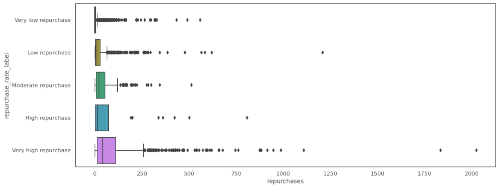
Boxplots of the repurchase rate labels show that the majority of orders are small, but there is a larger spread on some SKUs, plus some outliers on the lower repurchase rate items.
sns.boxplot(x="repurchases", y="repurchase_rate_label", data=df, palette="husl", orient='h')
<matplotlib.axes._subplots.AxesSubplot at 0x7f5630c52070>
Binning bulk purchase rate data
We can use the same binning approach on the bulk purchase rate data to assign labels to each SKU based on the number of times the SKU is purchased individually or in larger volumes.
def get_bulk_purchase_rate_label(df):

    labels = ['Very low bulk',
              'Low bulk',
              'Moderate bulk',
              'High bulk',
              'Very high bulk']
    df['bulk_purchase_rate_label'] = pd.cut(df['bulk_purchase_rate'],
                                          bins=5,
                                          labels=labels)
    return df
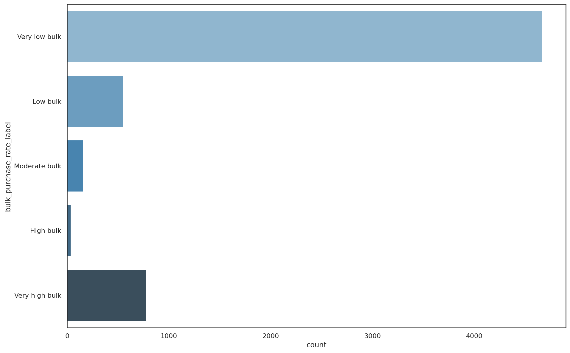
Running this function and examining the data shows that 75% of SKUs are purchased individually or in very low bulk quantities. Only 37 SKUs (0.6%) are purchased in high bulk, 2.6% are purchased in moderate bulk, and 8.86% are purchased in low bulk. Encouragingly, 12.6% are bought in very high bulk, so there are some opportunities here to try and get customers to buy more through promotions or bundling.
df = get_bulk_purchase_rate_label(df)
df['bulk_purchase_rate_label'].value_counts()
Very low bulk     4666
Very high bulk     780
Low bulk           549
Moderate bulk      162
High bulk           37
Name: bulk_purchase_rate_label, dtype: int64
f, ax = plt.subplots(figsize=(15, 10))
sns.countplot(y="bulk_purchase_rate_label", data=df, palette="Blues_d")
<matplotlib.axes._subplots.AxesSubplot at 0x7f56308faa00>
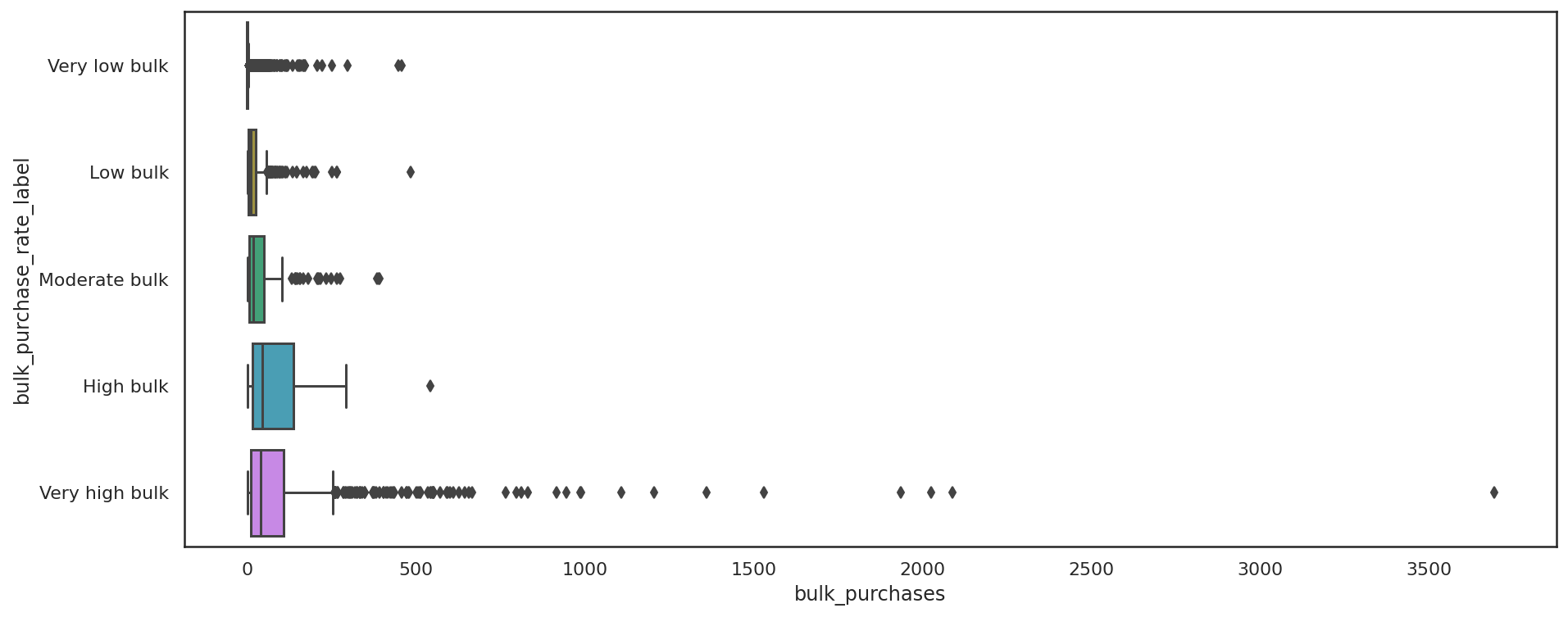
Boxplots of the bulk purchase rate for each label show the typical spread and the outliers. Even among the lower volume SKUs, there are some larger orders.
sns.boxplot(x="bulk_purchases", y="bulk_purchase_rate_label", data=df, palette="husl", orient='h')
<matplotlib.axes._subplots.AxesSubplot at 0x7f562fcb4400>
Create a combined label
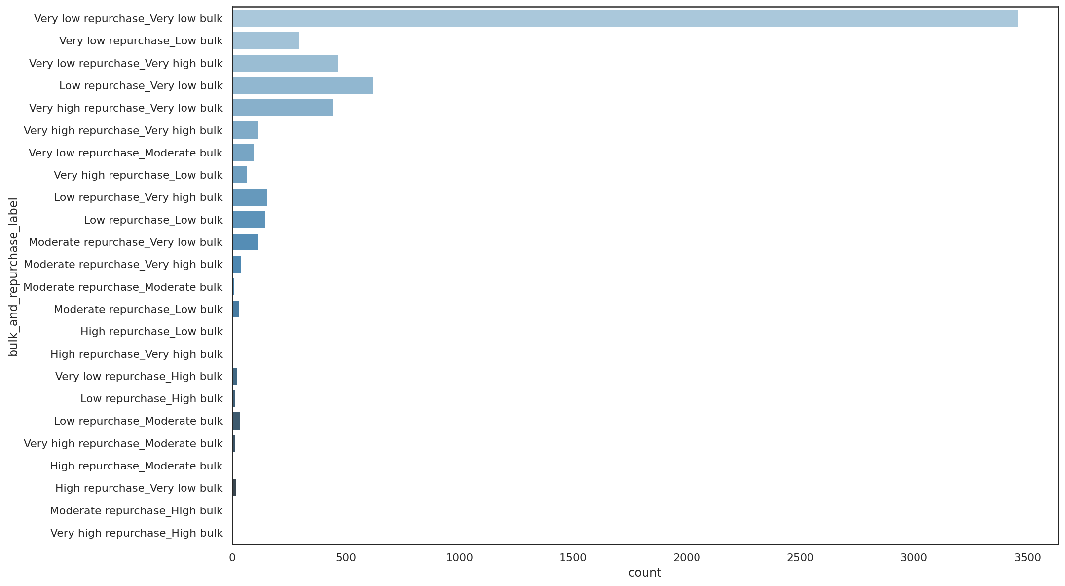
Finally, we can concatenate the two labels together to form a new feature which merges the repurchase rate data with the bulk purchase rate data. This is a good way to understand the types of products sold by the retailer. There’s a mixture of one-off purchases sold individually comprising the majority of units, followed by some one-offs purchased in bulk.
df['bulk_and_repurchase_label'] = df['repurchase_rate_label'].astype(str) +\
                            '_' + df['bulk_purchase_rate_label'].astype(str)
df.bulk_and_repurchase_label.value_counts()
Very low repurchase_Very low bulk      3461
Low repurchase_Very low bulk            624
Very low repurchase_Very high bulk      468
Very high repurchase_Very low bulk      446
Very low repurchase_Low bulk            296
Low repurchase_Very high bulk           154
Low repurchase_Low bulk                 147
Moderate repurchase_Very low bulk       116
Very high repurchase_Very high bulk     115
Very low repurchase_Moderate bulk        97
Very high repurchase_Low bulk            68
Moderate repurchase_Very high bulk       40
Low repurchase_Moderate bulk             37
Moderate repurchase_Low bulk             33
Very low repurchase_High bulk            22
High repurchase_Very low bulk            19
Very high repurchase_Moderate bulk       16
Low repurchase_High bulk                 13
Moderate repurchase_Moderate bulk        10
High repurchase_Low bulk                  5
High repurchase_Very high bulk            3
High repurchase_Moderate bulk             2
Very high repurchase_High bulk            1
Moderate repurchase_High bulk             1
Name: bulk_and_repurchase_label, dtype: int64
We can use Seaborn to visualise these numbers to see where the product portfolio sits in terms of product consumption and repurchase rate.
f, ax = plt.subplots(figsize=(15, 10))
sns.countplot(y="bulk_and_repurchase_label", data=df, palette="Blues_d")
<matplotlib.axes._subplots.AxesSubplot at 0x7f5630dcfbb0>
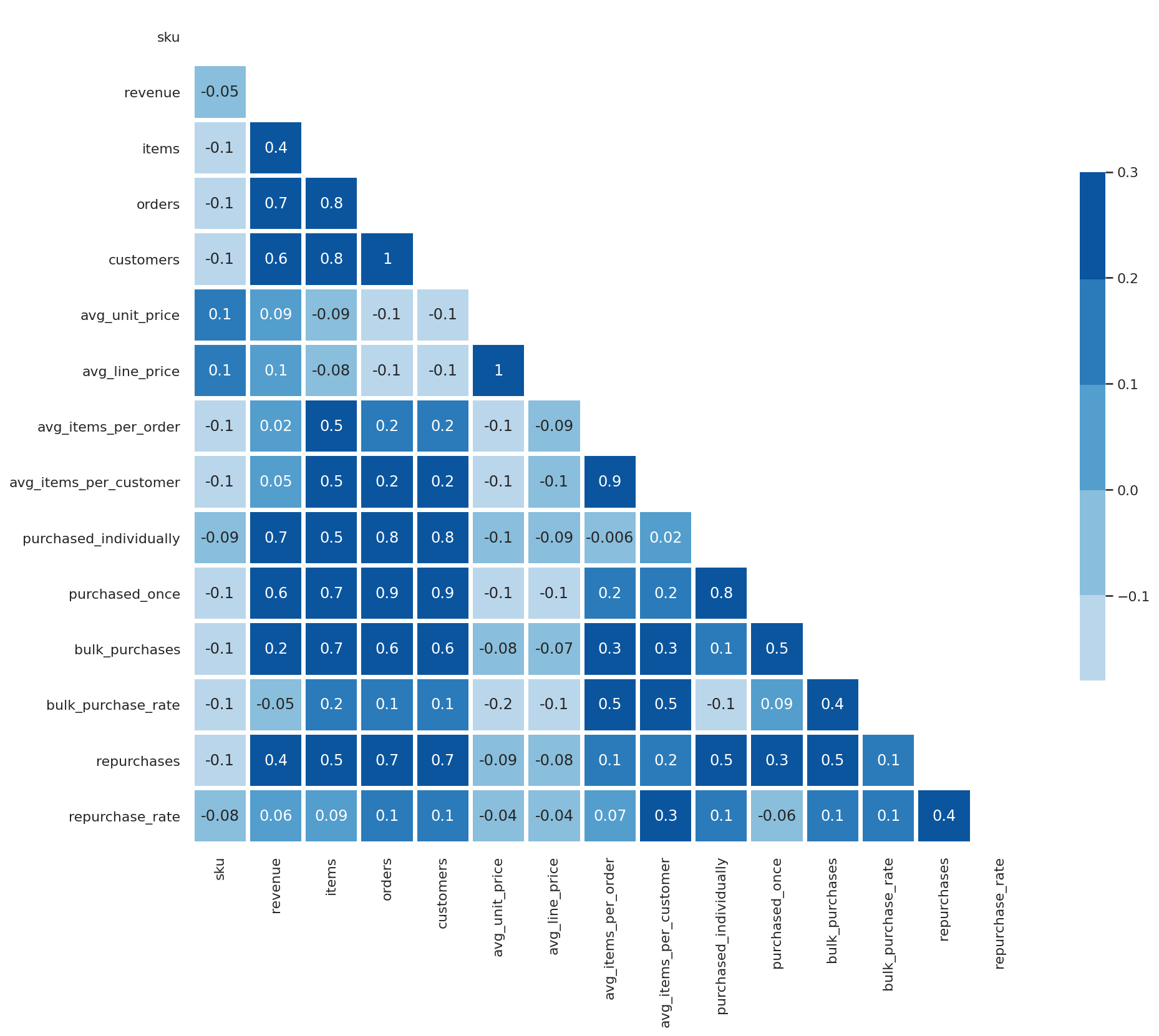
Examine correlations
Domain knowledge would likely be required to interpret whether the labels assigned were an issue or not. However, using a Pearson correlation matrix visualisation can show us the relationships between the metrics we’ve calculated.
sns.set_theme(style="white")
corr = df.corr()
mask = np.triu(df.corr())
f, ax = plt.subplots(figsize=(15, 15))
cmap = sns.color_palette("Blues")

sns.heatmap(corr,
            annot=True,
            fmt='.1g',
            mask=mask,
            cmap=cmap,
            vmax=.3,
            center=0,
            square=True,
            linewidths=3,
            cbar_kws={"shrink": .5}
           )
<matplotlib.axes._subplots.AxesSubplot at 0x7f562d59a790>
Some of the observations in here are obvious. The items that get repurchased in future orders are also often purchased in multiples in the same order, which suggests a multi-pack or bulk discount approach could work on some SKUs. As you’d imagine, the items that get frequently repurchased also tend to be cheaper lines.
df[df.columns[1:]].corr()['repurchase_rate'][:].sort_values(ascending=False).to_frame()
| repurchase_rate | |
|---|---|
| repurchase_rate | 1.000000 |
| repurchases | 0.410568 |
| avg_items_per_customer | 0.268418 |
| orders | 0.134656 |
| bulk_purchase_rate | 0.131190 |
| customers | 0.108661 |
| purchased_individually | 0.102367 |
| bulk_purchases | 0.100476 |
| items | 0.090003 |
| avg_items_per_order | 0.065705 |
| revenue | 0.061514 |
| avg_line_price | -0.037987 |
| avg_unit_price | -0.044577 |
| purchased_once | -0.061466 |
Examining the Pearson correlations for the bulk_purchase_rate against the other columns shows that overlap with repurchase rate again.
df[df.columns[1:]].corr()['bulk_purchase_rate'][:].sort_values(ascending=False).to_frame()
| bulk_purchase_rate | |
|---|---|
| bulk_purchase_rate | 1.000000 |
| avg_items_per_order | 0.502609 |
| avg_items_per_customer | 0.498400 |
| bulk_purchases | 0.378562 |
| items | 0.193714 |
| repurchase_rate | 0.131190 |
| orders | 0.123189 |
| customers | 0.119910 |
| repurchases | 0.118099 |
| purchased_once | 0.093817 |
Examine data by label
To further examine the relationship between the repurchase rate and the bulk purchase rate we can use a groupby() function with agg() to calculate some aggregate grouped statistics. These show us where the money is being made and from which type of SKU. Again, there could be some opportunities in here.
matrix = df.groupby('bulk_and_repurchase_label').agg(
    skus=('sku', 'nunique'),
    revenue=('revenue', 'sum'),
    orders=('orders', 'sum'),
    repurchases=('repurchases', 'sum'),
    repurchase_rate=('repurchase_rate', 'mean'),
    bulk_purchases=('bulk_purchases', 'sum'),
    bulk_purchase_rate=('bulk_purchase_rate', 'mean'),
    avg_line_price=('avg_line_price', 'mean'),
    avg_unit_price=('avg_unit_price', 'mean'),
    avg_items_per_order=('avg_items_per_order', 'mean'),
    avg_items_per_customer=('avg_items_per_customer', 'mean'),
).sort_values(by='revenue').reset_index()

matrix
| bulk_and_repurchase_label | skus | revenue | orders | repurchases | repurchase_rate | bulk_purchases | |
|---|---|---|---|---|---|---|---|
| 0 | High repurchase_Moderate bulk | 2 | 506.36 | 29 | 20.0 | 0.688095 | 13.0 |
| 1 | Very high repurchase_High bulk | 1 | 620.65 | 28 | 28.0 | 1.000000 | 21.0 |
| 2 | Moderate repurchase_High bulk | 1 | 1032.81 | 78 | 33.0 | 0.423077 | 47.0 |
| 3 | High repurchase_Very high bulk | 3 | 10025.72 | 384 | 242.0 | 0.673109 | 384.0 |
| 4 | Low repurchase_High bulk | 13 | 14198.55 | 1677 | 483.0 | 0.302736 | 1096.0 |
| 5 | Moderate repurchase_Moderate bulk | 10 | 16345.62 | 1282 | 602.0 | 0.464496 | 594.0 |
| 6 | Very high repurchase_Moderate bulk | 16 | 23596.03 | 2203 | 2203.0 | 1.000000 | 1043.0 |
| 7 | Very low repurchase_High bulk | 22 | 28129.11 | 2908 | 328.0 | 0.110200 | 2069.0 |
| 8 | Moderate repurchase_Low bulk | 33 | 62954.23 | 3000 | 1426.0 | 0.475055 | 843.0 |
| 9 | Very low repurchase_Moderate bulk | 97 | 74185.04 | 7652 | 1008.0 | 0.081755 | 3726.0 |
| 10 | High repurchase_Very low bulk | 19 | 105724.67 | 1919 | 1248.0 | 0.663566 | 230.0 |
| 11 | Low repurchase_Moderate bulk | 37 | 112949.27 | 5272 | 1418.0 | 0.272431 | 2573.0 |
| 12 | High repurchase_Low bulk | 5 | 126452.96 | 2441 | 1648.0 | 0.664788 | 606.0 |
| 13 | Very high repurchase_Low bulk | 68 | 132247.77 | 7641 | 7641.0 | 1.000000 | 2005.0 |
| 14 | Moderate repurchase_Very high bulk | 40 | 150596.85 | 5385 | 2601.0 | 0.477635 | 5385.0 |
| 15 | Low repurchase_Low bulk | 147 | 276827.23 | 13926 | 4037.0 | 0.284915 | 3953.0 |
| 16 | Very low repurchase_Low bulk | 296 | 303311.46 | 20751 | 2540.0 | 0.089262 | 5800.0 |
| 17 | Very high repurchase_Very high bulk | 115 | 314509.14 | 16392 | 16392.0 | 1.000000 | 16392.0 |
| 18 | Low repurchase_Very high bulk | 154 | 381045.32 | 22169 | 6177.0 | 0.279386 | 22048.0 |
| 19 | Moderate repurchase_Very low bulk | 116 | 519872.60 | 10959 | 4972.0 | 0.475866 | 1135.0 |
| 20 | Very low repurchase_Very high bulk | 468 | 711090.65 | 44021 | 5618.0 | 0.075183 | 43815.0 |
| 21 | Very high repurchase_Very low bulk | 446 | 1477897.79 | 42174 | 42173.0 | 0.999626 | 3234.0 |
| 22 | Low repurchase_Very low bulk | 624 | 2620426.54 | 59266 | 16206.0 | 0.279627 | 5260.0 |
| 23 | Very low repurchase_Very low bulk | 3461 | 9327054.06 | 179699 | 17923.0 | 0.051272 | 9537.0 |
Next steps
Now we’ve got our products labeled, and we have metrics identifying how customers commonly purchase them, some further work is required to extract some business value from the data. Here’s what I’d suggest, based on the findings above:
- Go back and add in the brand, product type or product category and re-run the analysis. Certain product types or product categories are likely to see more volume purchasing and more repeat purchasing than others.
- Are some products in the same product category, or the same product type showing different levels of volume purchasing or repeat purchasing? Are the products priced correctly? Are they appearing in product recommendations? Can product inter-linking be improved?
- For the products sold in multiples and that are repurchased, can multi-packs be created to try and increase basket sizes and values? Can you offer customers a discount to get them to “supersize” their order, either on the product page or at the basket?
- What is the average repurchase rate for each product type, product category and brand? Are some brands or products less popular than others? Is that correlated with review ratings? Should they be removed from the range?
- Can you combine the data with a cohort analysis? Can you measure whether recipients of a specific promotion were influenced to repurchase a product or brand again following an offer?
- If you know that certain customers frequently repurchase a particular product, can you persuade them to switch brands to a more profitable premium product?
- What do your best customers buy? Do you sell enough items that cause customers to buy again and again? Do the data suggest you have range gaps you need to fill?
There are probably loads of other things you could do with these data. Please let me know below if you have any other interesting applications.
Matt Clarke, Sunday, March 14, 2021


Other posts you might like

How to use the Pandas truncate() function
Have you ever needed to chop the top or bottom off a Pandas dataframe, or extract a specific section from the middle? If so, there’s a Pandas function called truncate()...

How to use Spacy for noun phrase extraction
Noun phrase extraction is a Natural Language Processing technique that can be used to identify and extract noun phrases from text. Noun phrases are phrases that function grammatically as nouns...
