How to analyse product replenishment
By identifying products that are regularly replenished and contacting customers when they are running low via replenishment emails, you can generate extra sales.

Subscription commerce was all the rage for a while, but it’s not really become as popular as many in ecommerce perhaps envisaged. While we may have subscriptions for certain things, most of us have continued to buy consumable products in the same way - by replenishing them whenever we run out.
Online retailers are wise to this common behaviour, and many create specific product replenishment email campaigns to target such customers. According to some marketing studies, these product replenishment emails can have the highest click through rates of any marketing automation emails, so they’re worth adding to your email marketing arsenal.
Product replenishment email campaigns
Product replenishment emails aim to contact each customer just before they are due to replenish a given product and give them with a gentle reminder to buy some more before they run out. They work because they’re timely and relevant. However, replenishment campaigns are harder to get right than you might first imagine, because customers all behave in slightly different ways.
| Volume purchased | Customers who buy a product in bulk may well need to stock up again less frequently than those who purchase smaller quantities more frequently. Similarly, an individual customer who usually purchases, say, a 2kg pack of protein powder which lasts them a week, might not need to purchase again at their usual interval if their last order was for a 10kg sack. |
| Consumption rate | Different people have different rates of product consumption, so they won't all replenish their products at the same rates. The mean time to replenish a given product might be 30 days, but some customers will use the product more quickly and need to replenish weekly, while for others their pack could last them months. |
| Seasonality | Replenishment rates can also be seasonal. Certain products get replenished only during certain seasons. For example, you might mince pies several times in the run up to Christmas, but try finding them in the summer... |
| Product type | Some products are just not replenished. For example, electrical appliances and gadgets tend to have a longer lifetime and customers rarely need more than one. By the time the product requires replacement, it's usually obsolete and has to be replaced with an alternative of the same general type. |
In this project, I’ll show you how you can use Pandas to calculate product replenishment rates for each of your products and calculate the average time it takes customers to replenish them. For simple products, the data could be used as-is to power basic product replenishment campaigns, but they also serve as the raw features for product replenishment campaign models.
Load the packages
First, open a Jupyter notebook and import the pandas, numpy, and seaborn packages. You’ll likely already have these installed, but if you don’t you can install them via the PyPi package manager by entering pip3 install package-name in your terminal or !pip3 install package-name in a cell in your Jupyter notebook.
import pandas as pd
import numpy as np
import seaborn as sns
%config InlineBackend.figure_format = 'retina'
sns.set_context('notebook')
sns.set(rc={'figure.figsize':(15, 6)})
Load the data
Next, load up your dataset of transaction items. I’m using the Online Retail dataset from the UCI Machine Learning Repository. This is widely used for demonstrations in ecommerce data science and includes a wide range of regularly purchased items from an online retailer selling party supplies. This includes a number of items that regularly get repurchased.
To tidy up the data, I have renamed the columns, and importantly, I have ordered the data in descending order of the order_date column. If you miss this vital step, you’ll get nonsensical results, since everything we’re doing relies on the data being ordered chronologically.
df = pd.read_csv('online_retail.csv',
                 names=['order_id', 'sku', 'description', 'quantity', 'order_date', 'unit_price', 'customer_id', 'country'],
                 skiprows=1).sort_values(by=['order_date'], ascending=False)
df.head()
| order_id | sku | description | quantity | order_date | unit_price | customer_id | country | |
|---|---|---|---|---|---|---|---|---|
| 541908 | 581587 | 22138 | BAKING SET 9 PIECE RETROSPOT | 3 | 2011-12-09 12:50:00 | 4.95 | 12680.0 | France |
| 541901 | 581587 | 22367 | CHILDRENS APRON SPACEBOY DESIGN | 8 | 2011-12-09 12:50:00 | 1.95 | 12680.0 | France |
| 541895 | 581587 | 22556 | PLASTERS IN TIN CIRCUS PARADE | 12 | 2011-12-09 12:50:00 | 1.65 | 12680.0 | France |
| 541896 | 581587 | 22555 | PLASTERS IN TIN STRONGMAN | 12 | 2011-12-09 12:50:00 | 1.65 | 12680.0 | France |
| 541897 | 581587 | 22728 | ALARM CLOCK BAKELIKE PINK | 4 | 2011-12-09 12:50:00 | 3.75 | 12680.0 | France |
Remove zero-value order lines
The second important thing we must do is ensure that any zero-value order lines, such as returns or free gifts, are removed from the dataset. An item that arrived damaged or was faulty and has been replaced free of charge shouldn’t be confused with a genuine replenishment of the product, so this step is critical. I’ve done this twice - once using unit_price and once using quantity and then have checked the aggregate statistics using describe().
df = df[df['unit_price'] > 0]
df = df[df['quantity'] > 0]
df.describe()
| quantity | unit_price | customer_id | |
|---|---|---|---|
| count | 530104.000000 | 530104.000000 | 397884.000000 |
| mean | 10.542037 | 3.907625 | 15294.423453 |
| std | 155.524124 | 35.915681 | 1713.141560 |
| min | 1.000000 | 0.001000 | 12346.000000 |
| 25% | 1.000000 | 1.250000 | 13969.000000 |
| 50% | 3.000000 | 2.080000 | 15159.000000 |
| 75% | 10.000000 | 4.130000 | 16795.000000 |
| max | 80995.000000 | 13541.330000 | 18287.000000 |
Calculate each customer’s previous order date for each SKU
In order to calculate the average replenishment time for each SKU, our first step is to calculate the replenishment date for each customer-SKU combination. To do this, we’ll use the Pandas groupby() function and will pass it both the customer_id and the sku. We’ll then append the order_date column and use the shift() function to get the previous value from the order_date column using -1.
df['previous_sku_order_date'] = df.groupby(['customer_id', 'sku'])['order_date'].shift(-1)
To check that the date of each customer’s previous order for each SKU has been calculated correctly, we can filter our dataframe to look at a specific customer-SKU combination. Customer 12680 has purchased the SKU 22728 three times, first on August 18th 2011, then on September 27th 2011, and finally on December 9th 2011. For each purchase, we’ve correctly assigned the date of the previous order to the previous_sku_order_date column, and have a NaN when the purchase was a customer’s first for the given SKU.
df[(df['customer_id']==12680) & (df['sku']=='22728')].sort_values(by='order_date', ascending=True)
| order_id | sku | description | quantity | order_date | unit_price | customer_id | country | previous_sku_order_date | |
|---|---|---|---|---|---|---|---|---|---|
| 305794 | 563712 | 22728 | ALARM CLOCK BAKELIKE PINK | 4 | 2011-08-18 15:44:00 | 3.75 | 12680.0 | France | NaN |
| 362787 | 568518 | 22728 | ALARM CLOCK BAKELIKE PINK | 4 | 2011-09-27 12:53:00 | 3.75 | 12680.0 | France | 2011-08-18 15:44:00 |
| 541897 | 581587 | 22728 | ALARM CLOCK BAKELIKE PINK | 4 | 2011-12-09 12:50:00 | 3.75 | 12680.0 | France | 2011-09-27 12:53:00 |
Calculate the number of days to replenishment
Next, we’ll create a function to calculate the number of days between each of a customer’s orders of a given SKU. This takes three values: the original dataframe, the “before” date, and the “after” date. It then calculates the time delta - or the time difference between the two dates - and returns the number of days as an integer, that we can then assign to a new column.
def get_days_since_date(df, before_datetime, after_datetime):
    """Return a new column containing the difference between two dates in days.
    Args:
        df: Pandas DataFrame.
        before_datetime: Earliest datetime (will convert value)
        after_datetime: Latest datetime (will convert value)
    Returns:
        Days since previous date.
    """
    df = df.copy()
    df[before_datetime] = pd.to_datetime(df[before_datetime])
    df[after_datetime] = pd.to_datetime(df[after_datetime])

    diff = df[after_datetime] - df[before_datetime]
    return round(diff / np.timedelta64(1, 'D')).fillna(0).astype(int)
To run the function we simply pass in the values and assign the output to a new column in our original dataframe
called days_since_previous_sku_order. Running the sample() function returns a sample set of rows, so we can check that the function has worked correctly.
df['days_since_previous_sku_order'] = get_days_since_date(df, 'previous_sku_order_date', 'order_date')
df[['order_id','sku','previous_sku_order_date','days_since_previous_sku_order']].sample(5)
| order_id | sku | previous_sku_order_date | days_since_previous_sku_order | |
|---|---|---|---|---|
| 192073 | 553390 | 22705 | NaN | 0 |
| 487136 | 577768 | 90165B | NaN | 0 |
| 359404 | 568188 | 23326 | NaN | 0 |
| 382126 | 569898 | 21787 | NaN | 0 |
| 116800 | 546306 | 22308 | NaN | 0 |
Calculate aggregate statistics on product replenishment
Since certain items are rarely, if ever, replenished, we also need to calculate some product-level data to identify replenishment rates across the product catalogue. We wouldn’t want to inadvertently contact a customer to tell them their TV is running out, when it’s a non-replenished item… Instead, we’d likely want to mark these as non-replenished items that we ignore from our campaigns.
Arguably, there’s also a difference between something that is replenished because it runs out (i.e., protein powder, coffee, or dog food) and something that is repurchased because it’s needed again for a completely different purpose (i.e., batteries for a new product). However, figuring this out is likely to be something that may require human input.
To calculate these data we’ll create a helper function called get_replenishments() to which we’ll pass our
dataframe of transactional items. We’ll first calculate the number of times each SKU has been purchased by each
customer and store it in the dataframe. Then, we’ll count the number of times it’s been purchased once only.
Next, we’ll create an aggregation containing the SKUs from the dataframe and calculate a range of metrics for each one. Then we’ll join the selected fields from our original transaction items dataframe back to the SKUs dataframe and return the output.
def get_replenishments(df):

    df['times_purchased'] = df.groupby(['sku', 'customer_id'])['order_id'].transform('count')
    df['times_purchased'] = df['times_purchased'].fillna(0).astype(int)

    df['purchased_once'] = df[df['times_purchased']==1].groupby('sku')['order_id'].transform('count')
    df['purchased_once'] = df['purchased_once'].fillna(0).astype(int)

    df_skus = df.groupby('sku').agg(
        total_customers=('customer_id', 'nunique'),
        total_orders=('order_id', 'nunique'),
        total_quantity=('quantity', 'sum'),
        avg_quantity=('quantity', 'mean'),
        avg_price=('unit_price', 'mean'),
        avg_replenishment_days=('days_since_previous_sku_order', 'mean'),
        std_replenishment_days=('days_since_previous_sku_order', 'std'),
        max_replenishment_days=('days_since_previous_sku_order', 'max'),
    )

    df_skus['orders_per_customer'] = df_skus['total_orders'] / df_skus['total_customers']
    df_skus['items_per_customer'] = df_skus['total_quantity'] / df_skus['total_customers']

    df_subset = df[['sku', 'purchased_once']].sort_values(by='purchased_once', ascending=False)
    df_subset = df_subset.drop_duplicates('sku', keep='first')
    df_skus = df_skus.merge(df_subset, on='sku', how='left')

    df_skus['total_replenishments'] = df_skus['total_orders'] - df_skus['purchased_once']
    df_skus['replenishment_rate'] = df_skus['total_replenishments'] / df_skus['total_orders']

    return df_skus
Running the function and sorting the data in descending order of total_replenishments shows us a range of products
that are regularly purchased repeatedly by customers. While this is useful for powering our replenishment campaign
emails, it’s potentially also worth looking at how we might be able to acquire customers more likely to purchase
these SKUs, since they’re likely to have good customer lifetime values with this level of repeat purchasing.
df_skus = get_replenishments(df)
df_skus.sort_values(by='total_replenishments', ascending=False).head(20)
| sku | total_customers | total_orders | total_quantity | avg_quantity | avg_price | avg_replenishment_days | std_replenishment_days | max_replenishment_days | orders_per_customer | items_per_customer | purchased_once | total_replenishments | replenishment_rate | |
|---|---|---|---|---|---|---|---|---|---|---|---|---|---|---|
| 3387 | 85099B | 635 | 2089 | 48474 | 22.951705 | 2.485459 | 27.729640 | 47.914234 | 326 | 3.289764 | 76.337008 | 321 | 1768 | 0.846338 |
| 3407 | 85123A | 856 | 2198 | 37660 | 16.626932 | 3.116949 | 32.940397 | 55.590776 | 365 | 2.567757 | 43.995327 | 432 | 1766 | 0.803458 |
| 1310 | 22423 | 881 | 1988 | 13879 | 6.881011 | 13.976926 | 28.187407 | 53.463092 | 355 | 2.256527 | 15.753689 | 547 | 1441 | 0.724849 |
| 175 | 20725 | 532 | 1565 | 19553 | 12.258934 | 2.127373 | 29.196238 | 47.193996 | 305 | 2.941729 | 36.753759 | 253 | 1312 | 0.838339 |
| 2670 | 47566 | 708 | 1685 | 18295 | 10.723916 | 5.794273 | 21.480657 | 39.548225 | 307 | 2.379944 | 25.840395 | 420 | 1265 | 0.750742 |
| 1109 | 22197 | 407 | 1392 | 56921 | 39.916550 | 1.042468 | 24.587658 | 47.259088 | 357 | 3.420147 | 139.855037 | 194 | 1198 | 0.860632 |
| 1276 | 22383 | 434 | 1284 | 12552 | 9.466063 | 2.160392 | 27.868024 | 45.716550 | 301 | 2.958525 | 28.921659 | 199 | 1085 | 0.845016 |
| 3194 | 84879 | 678 | 1455 | 36461 | 24.486904 | 1.722290 | 33.314305 | 56.257717 | 364 | 2.146018 | 53.777286 | 373 | 1082 | 0.743643 |
| 177 | 20727 | 458 | 1273 | 12240 | 9.216867 | 2.098479 | 28.236446 | 49.529678 | 351 | 2.779476 | 26.724891 | 220 | 1053 | 0.827180 |
| 1279 | 22386 | 372 | 1218 | 21465 | 17.338449 | 2.596115 | 23.790792 | 43.689494 | 287 | 3.274194 | 57.701613 | 205 | 1013 | 0.831691 |
| 908 | 21931 | 333 | 1184 | 13654 | 11.406850 | 2.744837 | 22.206349 | 43.616718 | 297 | 3.555556 | 41.003003 | 186 | 998 | 0.842905 |
| 3914 | POST | 331 | 1126 | 3150 | 2.797513 | 31.076581 | 32.924512 | 44.244217 | 322 | 3.401813 | 9.516616 | 142 | 984 | 0.873890 |
| 1593 | 22720 | 640 | 1385 | 7493 | 5.355969 | 5.829292 | 26.709793 | 54.632458 | 334 | 2.164062 | 11.707812 | 412 | 973 | 0.702527 |
| 2056 | 23203 | 505 | 1231 | 20503 | 16.415532 | 2.274668 | 21.392314 | 33.670773 | 208 | 2.437624 | 40.600000 | 264 | 967 | 0.785540 |
| 1298 | 22411 | 375 | 1175 | 12602 | 10.589916 | 2.683807 | 21.716807 | 44.582990 | 337 | 3.133333 | 33.605333 | 224 | 951 | 0.809362 |
| 439 | 21212 | 635 | 1320 | 36419 | 26.583212 | 0.758431 | 23.559124 | 53.346187 | 339 | 2.078740 | 57.352756 | 429 | 891 | 0.675000 |
| 178 | 20728 | 479 | 1150 | 11817 | 10.065588 | 2.059353 | 26.731687 | 46.744654 | 294 | 2.400835 | 24.670146 | 269 | 881 | 0.766087 |
| 1275 | 22382 | 490 | 1157 | 10464 | 8.875318 | 2.008473 | 28.381679 | 51.915599 | 357 | 2.361224 | 21.355102 | 283 | 874 | 0.755402 |
| 2866 | 82482 | 410 | 1100 | 9006 | 8.106211 | 3.101656 | 27.913591 | 51.779763 | 356 | 2.682927 | 21.965854 | 230 | 870 | 0.790909 |
| 1599 | 22727 | 388 | 1051 | 7815 | 7.276536 | 4.389050 | 31.699255 | 56.129841 | 350 | 2.708763 | 20.141753 | 193 | 858 | 0.816365 |
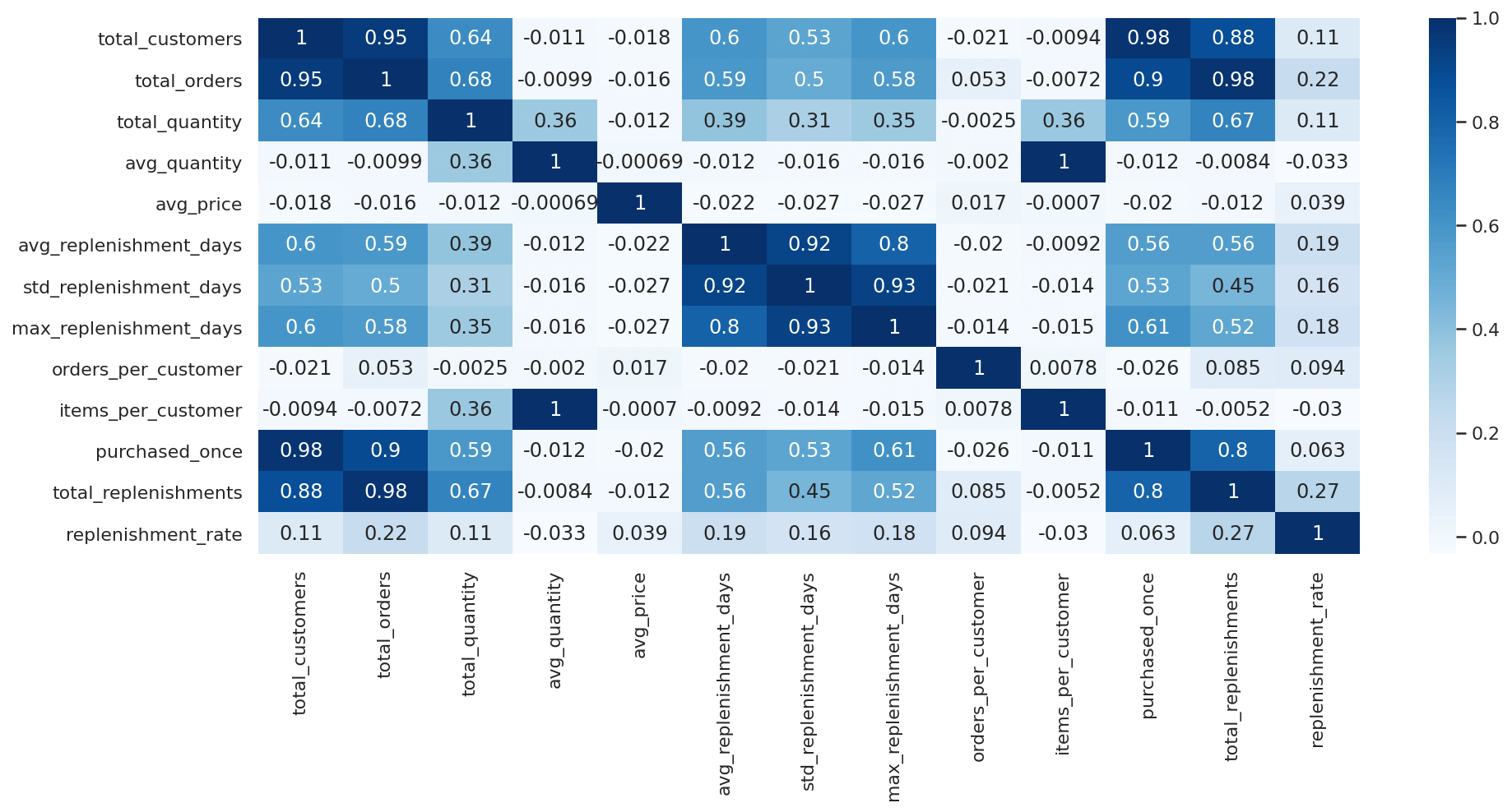
Examine correlations with replenishment time
Finally, just to sanity check our data and see if the assumptions we made earlier are correct, we can run a Pearson
correlation on the dataframe of SKU-level data. Before doing this, it’s worth zero-filling any inf values. You can
also plot the outputs to see how the data are correlated.
df_skus = df_skus.replace([np.inf, -np.inf], np.nan).fillna(value=0)
df_skus[df_skus.columns[1:]].corr()['avg_replenishment_days'][:].sort_values(ascending=False)
avg_replenishment_days    1.000000
std_replenishment_days    0.919889
max_replenishment_days    0.800298
total_customers           0.597277
total_orders              0.587021
purchased_once            0.563462
total_replenishments      0.560351
total_quantity            0.385017
replenishment_rate        0.193493
items_per_customer       -0.009193
avg_quantity             -0.012034
orders_per_customer      -0.020139
avg_price                -0.022023
Name: avg_replenishment_days, dtype: float64
sns.heatmap(df_skus.corr(), annot=True, cmap="Blues")
<AxesSubplot:>
We now have a SKU-level dataset that identifies the products that are regularly replenished, and those that are not,
so we can select or exclude them from our email marketing campaigns. Some retailers do use a metric such as
avg_replenishment_days to estimate when a customer is likely to purchase a product again. However, the most
accurate solution is likely to come from the creation of a product replenishment campaign model.
Replenishment campaign models typically use multiple linear regression and require a range of features to generate more accurate, personalised predictions. These features could include the SKU-level data above, plus the details on each individual customer-SKU relationship. With these data, they can then be trained to predict the number of days until each customer is likely to replenish their product.
Matt Clarke, Saturday, June 05, 2021


Other posts you might like

How to use the Pandas truncate() function
Have you ever needed to chop the top or bottom off a Pandas dataframe, or extract a specific section from the middle? If so, there’s a Pandas function called truncate()...

How to use Spacy for noun phrase extraction
Noun phrase extraction is a Natural Language Processing technique that can be used to identify and extract noun phrases from text. Noun phrases are phrases that function grammatically as nouns...
