How to create PDF reports in Python using Pandas and Gilfoyle

Picture by Matthew Osborn, Unsplash.

30 minutes to read

While reporting is often quite a useful way to stay on top of your data, it’s also something you can automate to save time, even if your reports include custom sections of analysis. To speed up the reporting process, I built a Python package that generates stylish looking PDF reports directly from Pandas dataframes.

My PDF report generator package, Gilfoyle, uses the Jinja2 templating library to first populate HTML templates configured to resemble PowerPoint presentations. It then uses Weasyprint to render the HTML to PDF, producing a customisable presentation that looks crisp on any screen.

It’s easy to use, allows you to use HTML and CSS to control the styling, and can be automated to save you more time. In this project I’ll show you how you can use it to create a monthly marketing report for each of your marketing channels based on your Google Analytics data.

Load the packages

First, open a Jupyter notebook and install my GAPandas and Gilfoyle packages by executing the below pip commands in a Jupyter cell, then import the packages. If you’re not pulling live data from the Google Analytics API, you can skip the GAPandas bit and just load your data straight into Pandas.

!pip3 install gapandas
!pip3 install gilfoyle

import pandas as pd
import gapandas as gp
from gilfoyle import report

Configure GAPandas

Next, configure some variables you can use within the Google Analytics API queries that define your JSON client secrets keyfile location, the Google Analytics view ID, and the start and end date for your reporting window. I use a 13-month period, since this shows the full year, plus the same month last year, allowing year-on-year change metrics to be calculated.

service = gp.get_service('client-secret.json')
view = '123456789'
start_date = '2020-02-01'
end_date = '2021-03-31'

Create a monthly report for all channels

Now GAPandas is set up, we can make use of the monthly_ecommerce_overview() helper function in GAPandas. You can write your own API queries out yourself if you like, but this makes the process much quicker and easier and cuts down massively on code repetition. The query below will fetch the key metrics for all sources and mediums and group the data by month and year.

df_all = gp.monthly_ecommerce_overview(service, view, start_date, end_date, segment=None, filters=None)
df_all.head(13)

	Period	Entrances	Sessions	Pageviews	Conversion rate	Revenue	AOV
0	March, 2021	23,376	23,376	37,238	0.00%	£0	£0.00
1	February, 2021	17,005	17,005	27,056	0.00%	£0	£0.00
2	January, 2021	18,682	18,683	30,110	0.00%	£0	£0.00
3	December, 2020	16,838	16,838	27,841	0.00%	£0	£0.00
4	November, 2020	18,671	18,671	30,893	0.00%	£0	£0.00
5	October, 2020	20,839	20,839	36,128	0.00%	£0	£0.00
6	September, 2020	23,158	23,159	39,408	0.00%	£0	£0.00
7	August, 2020	26,461	26,461	44,705	0.00%	£0	£0.00
8	July, 2020	30,106	30,106	49,009	0.00%	£0	£0.00
9	June, 2020	32,476	32,476	53,217	0.00%	£0	£0.00
10	May, 2020	28,552	28,553	48,794	0.00%	£0	£0.00
11	April, 2020	15,555	15,555	26,681	0.00%	£0	£0.00
12	March, 2020	17,029	17,029	29,515	0.00%	£0	£0.00

Create an organic search report

To create the data for your other marketing channels, it’s simply a case of passing in the required Google Analytics API filter parameter to the filters argument. Here, we’re setting the argument to ga:medium==organic to return only the data on organic search.

filter_organic = 'ga:medium==organic'
df_organic = gp.monthly_ecommerce_overview(service, view, start_date, end_date, segment=None, filters=filter_organic)
df_organic.head(13)

	Period	Entrances	Sessions	Pageviews	Conversion rate	Revenue	AOV
0	March, 2021	20,709	20,709	32,579	0.00%	£0	£0.00
1	February, 2021	15,205	15,205	23,843	0.00%	£0	£0.00
2	January, 2021	16,639	16,640	26,535	0.00%	£0	£0.00
3	December, 2020	14,996	14,996	24,550	0.00%	£0	£0.00
4	November, 2020	16,778	16,778	27,516	0.00%	£0	£0.00
5	October, 2020	18,609	18,609	32,051	0.00%	£0	£0.00
6	September, 2020	20,507	20,508	34,379	0.00%	£0	£0.00
7	August, 2020	23,282	23,282	39,194	0.00%	£0	£0.00
8	July, 2020	27,168	27,168	43,596	0.00%	£0	£0.00
9	June, 2020	29,048	29,048	47,109	0.00%	£0	£0.00
10	May, 2020	25,326	25,326	42,703	0.00%	£0	£0.00
11	April, 2020	13,256	13,256	22,123	0.00%	£0	£0.00
12	March, 2020	14,640	14,640	24,821	0.00%	£0	£0.00

Create a direct traffic report

We can now repeat the process for direct (or untracked) sessions, which are identified with the filter ga:medium==(none).

filter_direct = 'ga:medium==(none)'
df_direct = gp.monthly_ecommerce_overview(service, view, start_date, end_date, segment=None, filters=filter_direct)
df_direct.head(13)

	Period	Entrances	Sessions	Pageviews	Conversion rate	Revenue	AOV
0	March, 2021	2,444	2,444	4,202	0.00%	£0	£0.00
1	February, 2021	1,626	1,626	2,863	0.00%	£0	£0.00
2	January, 2021	1,854	1,854	3,212	0.00%	£0	£0.00
3	December, 2020	1,666	1,666	2,948	0.00%	£0	£0.00
4	November, 2020	1,698	1,698	3,067	0.00%	£0	£0.00
5	October, 2020	1,795	1,795	3,395	0.00%	£0	£0.00
6	September, 2020	2,385	2,385	4,590	0.00%	£0	£0.00
7	August, 2020	2,919	2,919	5,099	0.00%	£0	£0.00
8	July, 2020	2,628	2,628	4,850	0.00%	£0	£0.00
9	June, 2020	3,175	3,175	5,640	0.00%	£0	£0.00
10	May, 2020	2,830	2,831	5,321	0.00%	£0	£0.00
11	April, 2020	1,949	1,949	3,746	0.00%	£0	£0.00
12	March, 2020	2,073	2,073	3,861	0.00%	£0	£0.00

Create an email traffic report

The way your email traffic is tracked may depend on the utm tracking parameters you’ve configured in your emails, but for my site, they all go neatly under the ga:medium==email tracking parameter.

filter_email = 'ga:medium==email'
df_email = gp.monthly_ecommerce_overview(service, view, start_date, end_date, segment=None, filters=filter_email)
df_email.head(13)

	Period	Entrances	Sessions	Pageviews	Conversion rate	Revenue	AOV
0	March, 2021	3	3	12	0.00%	£0	£0.00
1	February, 2021	3	3	72	0.00%	£0	£0.00
2	January, 2021	3	3	5	0.00%	£0	£0.00
3	December, 2020	19	19	57	0.00%	£0	£0.00
4	November, 2020	6	6	7	0.00%	£0	£0.00
5	October, 2020	7	7	7	0.00%	£0	£0.00
6	September, 2020	14	14	35	0.00%	£0	£0.00
7	August, 2020	8	8	18	0.00%	£0	£0.00
8	July, 2020	10	10	30	0.00%	£0	£0.00
9	June, 2020	13	13	80	0.00%	£0	£0.00
10	May, 2020	13	13	41	0.00%	£0	£0.00
11	April, 2020	25	25	104	0.00%	£0	£0.00
12	March, 2020	30	30	234	0.00%	£0	£0.00

Create a referral report

Finally, since there’s minimal social or paid search activity on this site, I’ve pulled in the referral traffic from other sites linking in. You can, of course, make these as specific and granular as you want by adding more complex filters or by passing in a segment API query argument.

filter_referral = 'ga:medium==referral'
df_referral = gp.monthly_ecommerce_overview(service, view, start_date, end_date, segment=None, filters=filter_referral)
df_referral.head(13)

	Period	Entrances	Sessions	Pageviews	Conversion rate	Revenue	AOV
0	March, 2021	220	220	445	0.00%	£0	£0.00
1	February, 2021	168	168	271	0.00%	£0	£0.00
2	January, 2021	186	186	358	0.00%	£0	£0.00
3	December, 2020	157	157	286	0.00%	£0	£0.00
4	November, 2020	189	189	303	0.00%	£0	£0.00
5	October, 2020	426	426	670	0.00%	£0	£0.00
6	September, 2020	252	252	404	0.00%	£0	£0.00
7	August, 2020	252	252	394	0.00%	£0	£0.00
8	July, 2020	300	300	533	0.00%	£0	£0.00
9	June, 2020	240	240	388	0.00%	£0	£0.00
10	May, 2020	383	383	729	0.00%	£0	£0.00
11	April, 2020	324	324	707	0.00%	£0	£0.00
12	March, 2020	286	286	599	0.00%	£0	£0.00

Assemble your report

Now we’ve got our data into Pandas, we can move on to the creation of the PDF itself, which is done using my Gilfoyle package. To use Gilfoyle, we first instantiate the Report class and tell it the name of our output file, which I’ve called example.pdf, and then use get_payload() to obtain the initial payload.

pdf = report.Report(output='example.pdf')
payload = pdf.get_payload()

The get_payload() function returns a Python dictionary, which we can see in its empty form below. All our later functions basically populate this dictionary with pages, which get passed to Gilfoyle and used to render the reports using specially named variables that map to placeholders in the template.

payload

{'report': {}, 'pages': []}

Add a chapter page

For our first page, we’ll add a chapter cover using the add_page() function. We pass in the original payload dictionary from above, define the page_type as a chapter and set the page_title to “Example report”, and the page_subheading to “March 2021”. We reassign the output of add_page() back to the payload dictionary. If you print this, you’ll see that a page has been added to the pages list, which contains the placeholder values for our template.

payload = pdf.add_page(payload,
                       page_type='chapter',
                       page_title='Example report',
                       page_subheading='March 2021')

payload

{'report': {},
 'pages': [{'page_type': 'chapter',
   'page_layout': None,
   'page_title': 'Example report',
   'page_subheading': 'March 2021',
   'page_commentary': None,
   'page_message': None,
   'page_notification': None,
   'page_metrics': None,
   'page_dataframe': None,
   'page_visualisation': None,
   'page_background': None}]}

Python PDF report chapter

Add a report

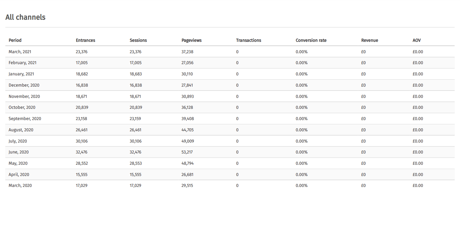
Next, we’ll take our df_all dataframe containing the Google Analytics data for all channels, and add it to a report. To do this, we repeat the process above but set the page_type to report, and the layout to simple. We then pass the df_all dataframe to the page_dataframe value. I’ve set this to head(13) so it displays the first 13 rows in the dataframe.

payload = pdf.add_page(payload,
                       page_type='report',
                       page_layout='simple',
                       page_title='All channels',
                       page_dataframe=df_all.head(13))

If you display the revised payload returned from the last add_page() function, you’ll notice that our new page has been added to the pages list in the dictionary. Gilfoyle has converted the original Pandas dataframe into an HTML table, added some styling elements to improve its appearance, and written it back to the dictionary, so it can be inserted into the template.

payload

{'report': {},
 'pages': [{'page_type': 'chapter',
   'page_layout': None,
   'page_title': 'Example report',
   'page_subheading': 'March 2021',
   'page_commentary': None,
   'page_message': None,
   'page_notification': None,
   'page_metrics': None,
   'page_dataframe': None,
   'page_visualisation': None,
   'page_background': None},
  {'page_type': 'report',
   'page_layout': 'simple',
   'page_title': 'All channels',
   'page_subheading': None,
   'page_commentary': None,
   'page_message': None,
   'page_notification': None,
   'page_metrics': None,
   'page_dataframe': '<table border="1" class="dataframe dataframe table is-striped is-fullwidth">\n  <thead>\n    <tr style="text-align: right;">\n      <th>Period</th>\n      <th>Entrances</th>\n      <th>Sessions</th>\n      <th>Pageviews</th>\n      <th>Transactions</th>\n      <th>Conversion rate</th>\n      <th>Revenue</th>\n      <th>AOV</th>\n    </tr>\n  </thead>\n  <tbody>\n    <tr>\n      <td>March, 2021</td>\n      <td>23,376</td>\n      <td>23,376</td>\n      <td>37,238</td>\n      <td>0</td>\n      <td>0.00%</td>\n      <td>£0</td>\n      <td>£0.00</td>\n    </tr>\n    <tr>\n      <td>February, 2021</td>\n      <td>17,005</td>\n      <td>17,005</td>\n      <td>27,056</td>\n      <td>0</td>\n      <td>0.00%</td>\n      <td>£0</td>\n      <td>£0.00</td>\n    </tr>\n    <tr>\n      <td>January, 2021</td>\n      <td>18,682</td>\n      <td>18,683</td>\n      <td>30,110</td>\n      <td>0</td>\n      <td>0.00%</td>\n      <td>£0</td>\n      <td>£0.00</td>\n    </tr>\n    <tr>\n      <td>December, 2020</td>\n      <td>16,838</td>\n      <td>16,838</td>\n      <td>27,841</td>\n      <td>0</td>\n      <td>0.00%</td>\n      <td>£0</td>\n      <td>£0.00</td>\n    </tr>\n    <tr>\n      <td>November, 2020</td>\n      <td>18,671</td>\n      <td>18,671</td>\n      <td>30,893</td>\n      <td>0</td>\n      <td>0.00%</td>\n      <td>£0</td>\n      <td>£0.00</td>\n    </tr>\n    <tr>\n      <td>October, 2020</td>\n      <td>20,839</td>\n      <td>20,839</td>\n      <td>36,128</td>\n      <td>0</td>\n      <td>0.00%</td>\n      <td>£0</td>\n      <td>£0.00</td>\n    </tr>\n    <tr>\n      <td>September, 2020</td>\n      <td>23,158</td>\n      <td>23,159</td>\n      <td>39,408</td>\n      <td>0</td>\n      <td>0.00%</td>\n      <td>£0</td>\n      <td>£0.00</td>\n    </tr>\n    <tr>\n      <td>August, 2020</td>\n      <td>26,461</td>\n      <td>26,461</td>\n      <td>44,705</td>\n      <td>0</td>\n      <td>0.00%</td>\n      <td>£0</td>\n      <td>£0.00</td>\n    </tr>\n    <tr>\n      <td>July, 2020</td>\n      <td>30,106</td>\n      <td>30,106</td>\n      <td>49,009</td>\n      <td>0</td>\n      <td>0.00%</td>\n      <td>£0</td>\n      <td>£0.00</td>\n    </tr>\n    <tr>\n      <td>June, 2020</td>\n      <td>32,476</td>\n      <td>32,476</td>\n      <td>53,217</td>\n      <td>0</td>\n      <td>0.00%</td>\n      <td>£0</td>\n      <td>£0.00</td>\n    </tr>\n    <tr>\n      <td>May, 2020</td>\n      <td>28,552</td>\n      <td>28,553</td>\n      <td>48,794</td>\n      <td>0</td>\n      <td>0.00%</td>\n      <td>£0</td>\n      <td>£0.00</td>\n    </tr>\n    <tr>\n      <td>April, 2020</td>\n      <td>15,555</td>\n      <td>15,555</td>\n      <td>26,681</td>\n      <td>0</td>\n      <td>0.00%</td>\n      <td>£0</td>\n      <td>£0.00</td>\n    </tr>\n    <tr>\n      <td>March, 2020</td>\n      <td>17,029</td>\n      <td>17,029</td>\n      <td>29,515</td>\n      <td>0</td>\n      <td>0.00%</td>\n      <td>£0</td>\n      <td>£0.00</td>\n    </tr>\n  </tbody>\n</table>',
   'page_visualisation': None,
   'page_background': None}]}

Python PDF report simple layout

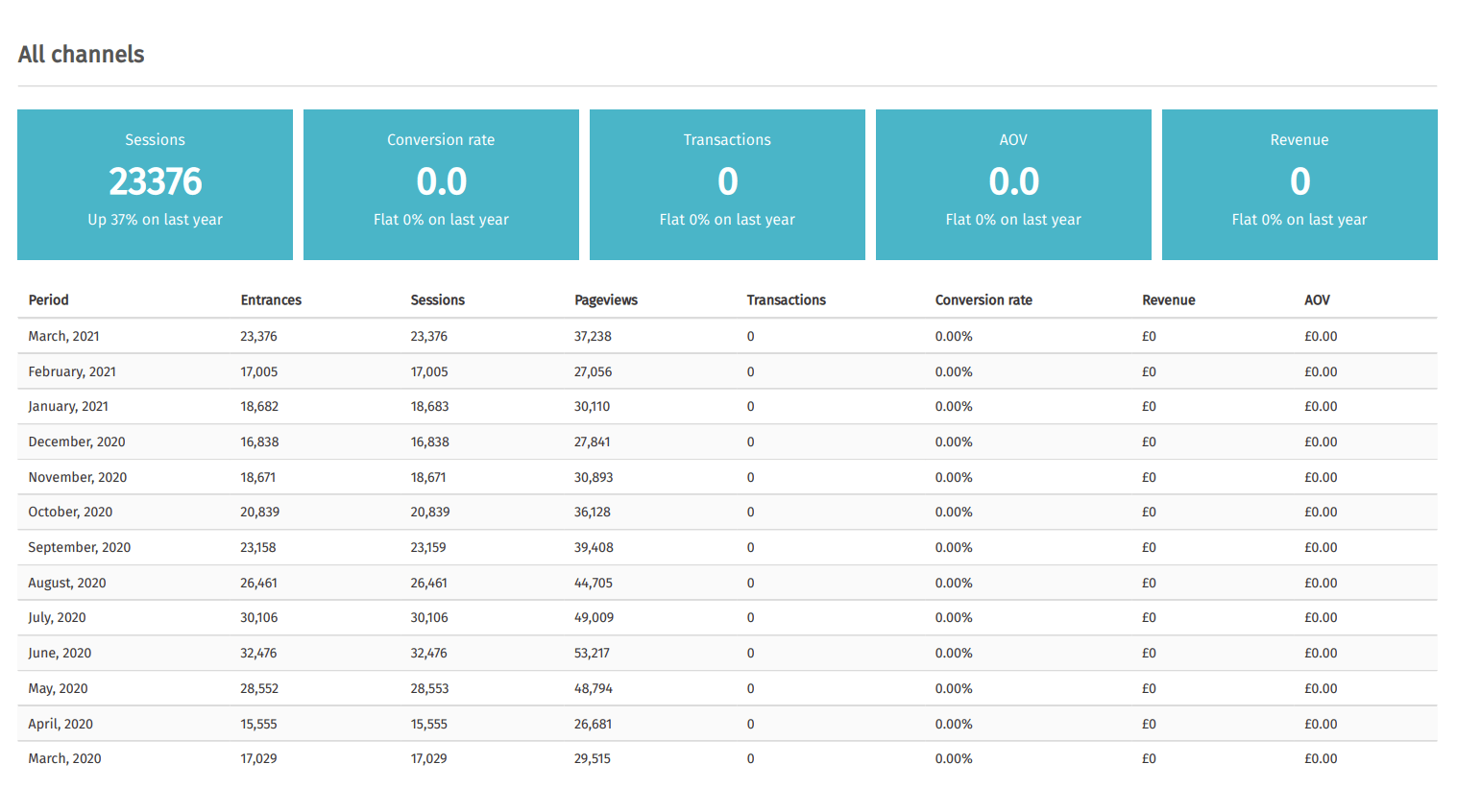
Adding metrics to your report

By default, if you create a report with the simple layout, Gilfoyle will just include a table. However, with a little extra effort you can also include metrics, and a range of other features. To add metrics we need to create a Python list called metrics which contains a dictionary for each metric “tile”. The metric tile requires a metric_title, i.e. Sessions, the value of the metric in the current period, and the value of the metric in the previous period.

For my report, I want to select a bunch of common metrics, and show the value in the most recent month, and the value in the same month last year. For the df_all dataframe, the value for the Sessions metric is located at loc[0], while the value for the same period last year is located at loc[12], so my individual metric data would look like this.

metrics = [
    pdf.add_metric_tile(
        metric_title='Sessions',
        metric_value_now=df_all['Sessions'].loc[0],
        metric_value_before=df_all['Sessions'].loc[12],
    )
]

If you print the output of the metrics list, you’ll see that Gilfoyle has included the metric_title as “Sessions”, and has extracted “23376” as the value in the last period, and has calculated that this is “Up 37% on last year”. All we need to do now, is repeat this process for each of the metrics we want to show on our report page.

metrics

[{'metric_title': 'Sessions',
  'metric_value': 23376,
  'metric_label': 'Up 37% on last year'}]

metrics = [
    pdf.add_metric_tile(
        metric_title='Sessions',
        metric_value_now=df_all['Sessions'].loc[0],
        metric_value_before=df_all['Sessions'].loc[12],
    ),
    pdf.add_metric_tile(
        metric_title='Conversion rate',
        metric_value_now=df_all['Conversion rate'].loc[0],
        metric_value_before=df_all['Conversion rate'].loc[12],
    ),
    pdf.add_metric_tile(
        metric_title='Transactions',
        metric_value_now=df_all['Transactions'].loc[0],
        metric_value_before=df_all['Transactions'].loc[12],
    ),
    pdf.add_metric_tile(
        metric_title='AOV',
        metric_value_now=df_all['AOV'].loc[0],
        metric_value_before=df_all['AOV'].loc[12],
    ),    
    pdf.add_metric_tile(
        metric_title='Revenue',
        metric_value_now=df_all['Revenue'].loc[0],
        metric_value_before=df_all['Revenue'].loc[12],
    ),
]

payload = pdf.add_page(payload,
                       page_type='report',
                       page_layout='simple',
                       page_title='All channels',
                       page_metrics=metrics,
                       page_dataframe=df_all.head(13))

Python PDF report metrics layout

Render a simple report

Now we’ve got a chapter and a simple report, one with metrics and one without, let’s render the output to PDF. When doing this, Gilfoyle will first create the template in HTML and then save the output to pdf. All you need to do is run create_report() and provide the payload dictionary and the output type.

pdf.create_report(payload, verbose=False, output='pdf')

Create a full report covering all channels

pdf = report.Report(output='marketing.pdf')
payload = pdf.get_payload()

payload = pdf.add_page(payload,
                       page_type='chapter',
                       page_title='Marketing report',
                       page_subheading='March 2021')

metrics = [
    pdf.add_metric_tile(
        metric_title='Sessions',
        metric_value_now=df_all['Sessions'].loc[0],
        metric_value_before=df_all['Sessions'].loc[12],
    ),
    pdf.add_metric_tile(
        metric_title='Conversion rate',
        metric_value_now=df_all['Conversion rate'].loc[0],
        metric_value_before=df_all['Conversion rate'].loc[12],
    ),
    pdf.add_metric_tile(
        metric_title='Transactions',
        metric_value_now=df_all['Transactions'].loc[0],
        metric_value_before=df_all['Transactions'].loc[12],
    ),
    pdf.add_metric_tile(
        metric_title='AOV',
        metric_value_now=df_all['AOV'].loc[0],
        metric_value_before=df_all['AOV'].loc[12],
    ),    
    pdf.add_metric_tile(
        metric_title='Revenue',
        metric_value_now=df_all['Revenue'].loc[0],
        metric_value_before=df_all['Revenue'].loc[12],
    ),
]

payload = pdf.add_page(payload,
                       page_type='report',
                       page_layout='simple',
                       page_title='All channels',
                       page_metrics=metrics,
                       page_dataframe=df_all.head(13))

metrics = [
    pdf.add_metric_tile(
        metric_title='Sessions',
        metric_value_now=df_organic['Sessions'].loc[0],
        metric_value_before=df_organic['Sessions'].loc[12],
    ),
    pdf.add_metric_tile(
        metric_title='Conversion rate',
        metric_value_now=df_organic['Conversion rate'].loc[0],
        metric_value_before=df_organic['Conversion rate'].loc[12],
    ),
    pdf.add_metric_tile(
        metric_title='Transactions',
        metric_value_now=df_organic['Transactions'].loc[0],
        metric_value_before=df_organic['Transactions'].loc[12],
    ),
    pdf.add_metric_tile(
        metric_title='AOV',
        metric_value_now=df_organic['AOV'].loc[0],
        metric_value_before=df_organic['AOV'].loc[12],
    ),    
    pdf.add_metric_tile(
        metric_title='Revenue',
        metric_value_now=df_organic['Revenue'].loc[0],
        metric_value_before=df_organic['Revenue'].loc[12],
    ),
]

payload = pdf.add_page(payload,
                       page_type='report',
                       page_layout='simple',
                       page_title='Organic search',
                       page_metrics=metrics,
                       page_dataframe=df_organic.head(13))

metrics = [
    pdf.add_metric_tile(
        metric_title='Sessions',
        metric_value_now=df_direct['Sessions'].loc[0],
        metric_value_before=df_direct['Sessions'].loc[12],
    ),
    pdf.add_metric_tile(
        metric_title='Conversion rate',
        metric_value_now=df_direct['Conversion rate'].loc[0],
        metric_value_before=df_direct['Conversion rate'].loc[12],
    ),
    pdf.add_metric_tile(
        metric_title='Transactions',
        metric_value_now=df_direct['Transactions'].loc[0],
        metric_value_before=df_direct['Transactions'].loc[12],
    ),
    pdf.add_metric_tile(
        metric_title='AOV',
        metric_value_now=df_direct['AOV'].loc[0],
        metric_value_before=df_direct['AOV'].loc[12],
    ),    
    pdf.add_metric_tile(
        metric_title='Revenue',
        metric_value_now=df_direct['Revenue'].loc[0],
        metric_value_before=df_direct['Revenue'].loc[12],
    ),
]

payload = pdf.add_page(payload,
                       page_type='report',
                       page_layout='simple',
                       page_title='Direct',
                       page_metrics=metrics,
                       page_dataframe=df_direct.head(13))

metrics = [
    pdf.add_metric_tile(
        metric_title='Sessions',
        metric_value_now=df_email['Sessions'].loc[0],
        metric_value_before=df_email['Sessions'].loc[12],
    ),
    pdf.add_metric_tile(
        metric_title='Conversion rate',
        metric_value_now=df_email['Conversion rate'].loc[0],
        metric_value_before=df_email['Conversion rate'].loc[12],
    ),
    pdf.add_metric_tile(
        metric_title='Transactions',
        metric_value_now=df_email['Transactions'].loc[0],
        metric_value_before=df_email['Transactions'].loc[12],
    ),
    pdf.add_metric_tile(
        metric_title='AOV',
        metric_value_now=df_email['AOV'].loc[0],
        metric_value_before=df_email['AOV'].loc[12],
    ),    
    pdf.add_metric_tile(
        metric_title='Revenue',
        metric_value_now=df_email['Revenue'].loc[0],
        metric_value_before=df_email['Revenue'].loc[12],
    ),
]

payload = pdf.add_page(payload,
                       page_type='report',
                       page_layout='simple',
                       page_title='Email',
                       page_metrics=metrics,
                       page_dataframe=df_email.head(13))

metrics = [
    pdf.add_metric_tile(
        metric_title='Sessions',
        metric_value_now=df_referral['Sessions'].loc[0],
        metric_value_before=df_referral['Sessions'].loc[12],
    ),
    pdf.add_metric_tile(
        metric_title='Conversion rate',
        metric_value_now=df_referral['Conversion rate'].loc[0],
        metric_value_before=df_referral['Conversion rate'].loc[12],
    ),
    pdf.add_metric_tile(
        metric_title='Transactions',
        metric_value_now=df_referral['Transactions'].loc[0],
        metric_value_before=df_referral['Transactions'].loc[12],
    ),
    pdf.add_metric_tile(
        metric_title='AOV',
        metric_value_now=df_referral['AOV'].loc[0],
        metric_value_before=df_referral['AOV'].loc[12],
    ),    
    pdf.add_metric_tile(
        metric_title='Revenue',
        metric_value_now=df_referral['Revenue'].loc[0],
        metric_value_before=df_referral['Revenue'].loc[12],
    ),
]

payload = pdf.add_page(payload,
                       page_type='report',
                       page_layout='simple',
                       page_title='Referral',
                       page_metrics=metrics,
                       page_dataframe=df_referral.head(13))

pdf.create_report(payload, verbose=False, output='pdf')

Here’s the report we generated as a PDF. In seconds, Gilfoyle has taken the outputs of our Pandas dataframes, which were created by querying your Google Analytics data, and has created a fairly attractive PDF report containing monthly data on each metric, as well as a range of metric tiles, which make it easier to see what’s improved and what hasn’t.

There’s loads more you can do with Gilfoyle, including adding in commentary, alert messages, graphs, and much more. This is just scratching the surface, but it should be plenty to get you up and running and should help you save valuable time building reports and presentations at work.

Matt Clarke, Saturday, April 24, 2021

Matt Clarke Matt is an Ecommerce and Marketing Director who uses data science to help in his work. Matt has a Master's degree in Internet Retailing (plus two other Master's degrees in different fields) and specialises in the technical side of ecommerce and marketing.