How to engineer customer purchase latency features
Learn how to engineer customer purchase latency features based on the time between each customer's orders so you can improve your model performance.

Purchase latency or customer latency is a measure of the number of days between a customer’s orders and is one of the most powerful features in many propensity and churn models. It’s based on the fact that the timing of each customer’s next order will fall somewhere around the mean of their usual gap between orders.
If a customer comes back to your store every 30 days on average, there will be a bit of standard deviation in the gaps between their orders, so they might order every 20-40 days. However, unless they only purchase seasonally, if it’s been 60 days since their last visit, there’s a higher probability that they’ve churned. On the other hand, if they only purchased 10 days ago, they’re unlikely to purchase again for at least a couple of weeks.
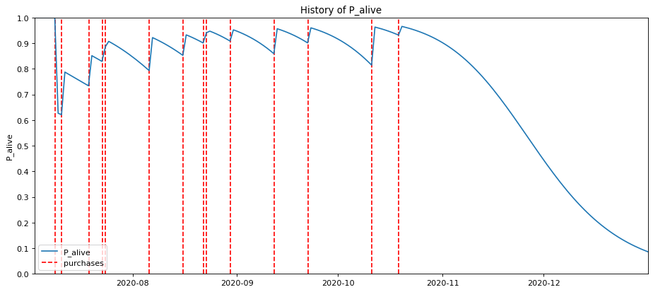
The chart above shows this in action. You can see that the customer doesn’t order exactly every X days. Instead, they have an average latency and will order a bit either side of this mean number. When the gap between their orders is small, and within their usual mean, the probability of them having churned is low, but when there’s been a longer gap, the chances of them having lapsed are far greater.
Making good use of latency metrics
While I’ve covered some more sophisticated models for predicting churn probability (such as the powerful BG/NBD model), here we’re specifically looking at the creation of model features for customer latency that you can use in other machine learning models. Latency features can prove extremely useful in these models, so it’s worth taking the time to engineer them.
In addition, in their raw form they can also help your sales teams understand the behaviour of their customers and help your marketing team focus their activities with greater accuracy. Here are a few practical ways you can use them:
-
Targeting customers who are due to order: When you know that a customer is due to order soon, you can target them with perfectly-timed marketing to try to entice them. Or, if you’re a B2B retailer, you may wish to call them.
-
Avoid contacting customers too soon: If you know a customer is within their normal mean latency, it’s less likely that they’ll order again immediately.
-
Reactivating lapsed customers: Once you know a customer has gone beyond their usual standard deviation in latency, you know their probability of still being a customer is rapidly falling, so you can target them with offers or contact them to try and re-engage them.
Load your transactional data
To calculate customer latency you only need three columns from your transactional dataset - the order ID, the customer ID, and the date of the order. The date column needs to be in a datetime format, so you may need to change the data type before you proceed.
import pandas as pd
import numpy as np

df_orders = pd.read_csv('orders.csv', low_memory=False)
df_orders['date_created'] = pd.to_datetime(df_orders['date_created'])
df_orders = df_orders[['order_id','customer_id','date_created','total_revenue']]
df_orders.sample(5)
| order_id | customer_id | date_created | total_revenue | |
|---|---|---|---|---|
| 66558 | 310352 | 126628 | 2020-10-04 11:49:09 | 62.37 |
| 4014 | 246882 | 122033 | 2017-06-24 15:30:30 | 49.00 |
| 61198 | 304992 | 114997 | 2020-05-19 10:09:28 | 123.43 |
| 12013 | 255142 | 89238 | 2017-11-07 22:45:54 | 56.00 |
| 56619 | 300413 | 81997 | 2020-02-05 12:36:03 | 30.69 |
df_orders.info()
<class 'pandas.core.frame.DataFrame'>
RangeIndex: 66988 entries, 0 to 66987
Data columns (total 4 columns):
 #   Column         Non-Null Count  Dtype
---  ------         --------------  -----
 0   order_id       66988 non-null  int64
 1   customer_id    66988 non-null  int64
 2   date_created   66988 non-null  datetime64[ns]
 3   total_revenue  66988 non-null  float64
dtypes: datetime64[ns](1), float64(1), int64(2)
memory usage: 2.0 MB
Remove any zero-value orders
Sometimes when customers buy an item it may get lost or damaged in the post, or it might develop a fault. In these cases, the company will issue a replacement free of charge. Since these don’t really represent actual orders placed by the customer, we need to filter them out.
df_orders = df_orders[df_orders['total_revenue'] > 0]
df_orders.sample(5)
| order_id | customer_id | date_created | total_revenue | |
|---|---|---|---|---|
| 20425 | 263835 | 119136 | 2018-04-15 13:01:21 | 57.99 |
| 19241 | 262612 | 119040 | 2018-03-24 12:03:58 | 49.99 |
| 21960 | 265426 | 124088 | 2018-05-11 10:58:41 | 54.99 |
| 41063 | 284857 | 119258 | 2019-04-04 06:57:07 | 52.00 |
| 59130 | 302924 | 79899 | 2020-03-18 12:01:23 | 58.43 |
Calculate the date of each previous order
To calculate the various latency metrics, the first step is to calculate the number of days between each of a customer’s orders. First, we’ll create a function called get_previous_value() which uses the Pandas shift() function to go back -1 to obtain the previous value in a sorted dataframe. By running this function we can assign the date of the previous order, if there was one, to a new column called prev_order_date.
def get_previous_value(df, group, column):
    """Group by a column and return the previous value of another column and assign value to a new column.
    Args:
        df: Pandas DataFrame.
        group: Column name to groupby
        column: Column value to return.
    Returns:
        Original DataFrame with new column containing previous value of named column.
    """
    df = df.copy()
    return df.groupby([group])[column].shift(-1)
df_orders = df_orders.sort_values(by=['date_created'], ascending=False)
df_orders['prev_order_date'] = get_previous_value(df_orders, 'customer_id', 'date_created')
df_orders.head()
| order_id | date_created | prev_order_date | |
|---|---|---|---|
| 66987 | 310781 | 2020-10-17 10:59:37 | 2020-09-09 18:31:06 |
| 66986 | 310780 | 2020-10-17 10:49:28 | 2020-08-22 13:20:48 |
| 66985 | 310779 | 2020-10-17 09:36:15 | 2020-06-27 08:52:23 |
| 66984 | 310778 | 2020-10-17 09:24:22 | 2020-08-13 08:33:41 |
| 66983 | 310777 | 2020-10-17 09:00:09 | 2020-02-27 18:41:40 |
Calculate the number of days between orders
Now we have the date of the current and previous orders, we can calculate the difference between the two days. We’ll create a helper function called get_days_since_date() that we can re-use. This takes the before and after dates and returns an integer containing the number of days difference.
def get_days_since_date(df, before_datetime, after_datetime):
    """Return a new column containing the difference between two dates in days.
    Args:
        df: Pandas DataFrame.
        before_datetime: Earliest datetime (will convert value)
        after_datetime: Latest datetime (will convert value)
    Returns:
        New column value
    """
    df = df.copy()
    df[before_datetime] = pd.to_datetime(df[before_datetime])
    df[after_datetime] = pd.to_datetime(df[after_datetime])

    diff = df[after_datetime] - df[before_datetime]
    return round(diff / np.timedelta64(1, 'D')).fillna(0).astype(int)
df_orders['days_since_prev_order'] = get_days_since_date(df_orders, 'prev_order_date', 'date_created')
df_orders.head()
| order_id | customer_id | date_created | total_revenue | prev_order_date | days_since_prev_order | |
|---|---|---|---|---|---|---|
| 66987 | 310781 | 139259 | 2020-10-17 10:59:37 | 61.41 | 2020-09-09 18:31:06 | 38 |
| 66986 | 310780 | 105029 | 2020-10-17 10:49:28 | 54.23 | 2020-08-22 13:20:48 | 56 |
| 66985 | 310779 | 122669 | 2020-10-17 09:36:15 | 241.53 | 2020-06-27 08:52:23 | 112 |
| 66984 | 310778 | 105986 | 2020-10-17 09:24:22 | 54.94 | 2020-08-13 08:33:41 | 65 |
| 66983 | 310777 | 134695 | 2020-10-17 09:00:09 | 54.95 | 2020-02-27 18:41:40 | 233 |
Calculating the order number
Next, we want to calculate the order number for each order placed by a customer. This has many uses and is worth storing in your data warehouse. For example, you can use it to identify new and returning customers and examine how their spending patterns change over time.
We’ll create a reusable function called get_cumulative_count() to calculate this. This will sort the dataframe by a given column, then group it by another column and return the cumulative count.
def get_cumulative_count(df, group, count_column, sort_column):
    """Get the cumulative count of a column based on a GroupBy.
    Args:
        :param df: Pandas DataFrame.
        :param group: Column to group by.
        :param count_column: Column to count.
        :param sort_column: Column to sort by.
    Returns:
        Cumulative count of the column.
    Usage:
        df['running_total'] = get_cumulative_count(df, 'customer_id', 'order_id', 'date_created')
    """
    df = df.sort_values(by=sort_column, ascending=True)
    return df.groupby([group])[count_column].cumcount()
Next, we’ll apply the get_cumulative_count() function to sort the column by the date_created, group by the customer_id, and return the cumulative count of the order_id column, giving us the order number for each order placed by each customer.
df_orders['order_number'] = get_cumulative_count(df_orders, 'customer_id', 'order_id', 'date_created')
df_orders[['order_id','order_number']].head()
| order_id | order_number | |
|---|---|---|
| 66987 | 310781 | 2 |
| 66986 | 310780 | 22 |
| 66985 | 310779 | 16 |
| 66984 | 310778 | 1 |
| 66983 | 310777 | 3 |
Create a dataframe of unique customers
Now we’ve calculated the latency metrics and stored them on the orders dataframe, we need to move to the next step and obtain calculations at the customer level. The first step is therefore to create a dataframe containing all of the unique customers in the orders dataframe.
df_customers = pd.DataFrame(df_orders['customer_id'].unique())
df_customers.columns = ['customer_id']
df_customers.head()
| customer_id | |
|---|---|
| 0 | 139259 |
| 1 | 105029 |
| 2 | 122669 |
| 3 | 105986 |
| 4 | 134695 |
Calculate frequency
df_frequency = df_orders.groupby('customer_id')['order_id'].nunique().reset_index()
df_frequency.columns = ['customer_id','frequency']
df_customers = df_customers.merge(df_frequency, on='customer_id')
df_customers.head()
| customer_id | frequency | |
|---|---|---|
| 0 | 139259 | 3 |
| 1 | 105029 | 23 |
| 2 | 122669 | 17 |
| 3 | 105986 | 2 |
| 4 | 134695 | 4 |
Calculate the overall average latency
To calculate the overall average latency for each customer we can use the Pandas, split, apply, combine technique. First we will group the data by the customer_id column and calculate the mean days_since_previous_order and cast the value to an integer to allow grouping. Then we’ll create a dataframe containing the column and the customer_id and we’ll merge it back onto the df_customers dataframe.
df_avg_latency = df_orders.groupby('customer_id')['days_since_prev_order'].mean().astype(int).reset_index()
df_avg_latency.columns = ['customer_id','avg_latency']
df_customers = df_customers.merge(df_avg_latency, on='customer_id')
df_customers.head()
| customer_id | frequency | avg_latency | |
|---|---|---|---|
| 0 | 139259 | 3 | 22 |
| 1 | 105029 | 23 | 54 |
| 2 | 122669 | 17 | 73 |
| 3 | 105986 | 2 | 32 |
| 4 | 134695 | 4 | 120 |
Calculate latency over recent periods
Customer purchase latency often changes. As customers become more established, latency tends to become lower, while as customers churn it becomes higher. A useful way of examining this is to calculate the average latency over 12 and 24 month periods. To do this, the first step is to create two dataframes - one for the past 12 months and one for the past 24 months, which we can do using timedelta().
df_orders_12m = df_orders[df_orders['date_created'] > ( pd.to_datetime('today') - \
                                       timedelta(days=365)).strftime('%Y-%m-%d')]

df_orders_24m = df_orders[df_orders['date_created'] > ( pd.to_datetime('today') - \
                                       timedelta(days=730)).strftime('%Y-%m-%d')]
Then we can repeat the split, apply, combine approach we used before but apply it to each of the date filtered dataframes in order to calculate the average purchase latency over 12 month and 24 month periods. Then we just assign the values to the df_customers dataframe.
df_avg_latency_12m = df_orders_12m.groupby('customer_id')['days_since_prev_order'].mean().astype(int).reset_index()
df_avg_latency_12m.columns = ['customer_id','avg_latency_12m']
df_customers = df_customers.merge(df_avg_latency_12m, on='customer_id')
df_customers.head()
| customer_id | frequency | avg_latency | avg_latency_12m | |
|---|---|---|---|---|
| 0 | 139259 | 3 | 22 | 22 |
| 1 | 105029 | 23 | 54 | 52 |
| 2 | 122669 | 17 | 73 | 168 |
| 3 | 105986 | 2 | 32 | 32 |
| 4 | 134695 | 4 | 120 | 214 |
df_avg_latency_24m = df_orders_24m.groupby('customer_id')['days_since_prev_order'].mean().astype(int).reset_index()
df_avg_latency_24m.columns = ['customer_id','avg_latency_24m']
df_customers = df_customers.merge(df_avg_latency_24m, on='customer_id')
df_customers.head()
| customer_id | frequency | avg_latency | avg_latency_12m | avg_latency_24m | |
|---|---|---|---|---|---|
| 0 | 139259 | 3 | 22 | 22 | 22 |
| 1 | 105029 | 23 | 54 | 52 | 56 |
| 2 | 122669 | 17 | 73 | 168 | 104 |
| 3 | 105986 | 2 | 32 | 32 | 32 |
| 4 | 134695 | 4 | 120 | 214 | 120 |
Calculate variation in customer latency
If we look at a random customer and examine their order latencies in the days_since_prev_order column, we see that they generally purchase every 80-114 days. If it’s been 10 days since their last order, the customer isn’t likely to purchase, but if it’s been 80-90 days, their order is imminent.
df_orders[df_orders['customer_id']==65427]
| order_id | customer_id | date_created | total_revenue | prev_order_date | days_since_prev_order | order_number | |
|---|---|---|---|---|---|---|---|
| 63724 | 307518 | 65427 | 2020-07-30 05:27:54 | 57.39 | 2020-04-17 20:32:19 | 103 | 12 |
| 60243 | 304037 | 65427 | 2020-04-17 20:32:19 | 60.45 | 2020-01-18 20:02:30 | 90 | 11 |
| 55820 | 299614 | 65427 | 2020-01-18 20:02:30 | 54.49 | 2019-10-18 07:47:24 | 93 | 10 |
| 51378 | 295172 | 65427 | 2019-10-18 07:47:24 | 54.99 | 2019-06-26 17:45:52 | 114 | 9 |
| 45835 | 289629 | 65427 | 2019-06-26 17:45:52 | 55.99 | 2019-03-07 14:38:57 | 111 | 8 |
| 39363 | 283157 | 65427 | 2019-03-07 14:38:57 | 54.99 | 2018-11-20 11:06:53 | 107 | 7 |
| 32997 | 276791 | 65427 | 2018-11-20 11:06:53 | 53.00 | 2018-08-26 12:41:18 | 86 | 6 |
| 28025 | 271701 | 65427 | 2018-08-26 12:41:18 | 54.99 | 2018-05-25 10:53:12 | 93 | 5 |
| 22770 | 266260 | 65427 | 2018-05-25 10:53:12 | 54.99 | 2018-02-21 08:35:10 | 93 | 4 |
| 17592 | 260914 | 65427 | 2018-02-21 08:35:10 | 53.99 | 2017-12-02 21:06:51 | 80 | 3 |
| 13535 | 256740 | 65427 | 2017-12-02 21:06:51 | 56.00 | 2017-09-01 06:46:31 | 93 | 2 |
| 8091 | 251089 | 65427 | 2017-09-01 06:46:31 | 55.99 | 2017-06-01 20:16:48 | 91 | 1 |
| 2598 | 245425 | 65427 | 2017-06-01 20:16:48 | 58.00 | NaT | 0 | 0 |
To calculate each customer’s minimum latency we need to ignore order zero, since there will be no latency on this order. Once we have these values, we can then calculate and round the minimum value and assign it back to the df_customers dataframe. Once we’ve done that, we can repeat the process to obtain the maximum latency.
df_orders_returning = df_orders[df_orders['order_number'] > 0]

df_min = df_orders_returning.groupby('customer_id')\
['days_since_prev_order'].min().astype(int).reset_index()

df_min.columns = ['customer_id','min_latency']
df_customers = df_customers.merge(df_min, on='customer_id')
df_max = df_orders_returning.groupby('customer_id')\
['days_since_prev_order'].max().astype(int).reset_index()

df_max.columns = ['customer_id','max_latency']
df_customers = df_customers.merge(df_max, on='customer_id')
df_customers[df_customers['customer_id']==65427]
| customer_id | frequency | avg_latency | avg_latency_12m | avg_latency_24m | min_latency | max_latency | |
|---|---|---|---|---|---|---|---|
| 2267 | 65427 | 13 | 88 | 95 | 100 | 80 | 114 |
Standard deviation will show us the amount of variation in the values for each customer. We can calculate this for each customer using the same split, apply, combine approach and utilise the std() function in Pandas. Examining our random sample customer shows that they have a standard deviation in their purchase latency of 10.3 days. Across 13 orders they’ve reordered every 80-114 days. By feeding these values into a regression model, we can predict when they’d be likely to order next.
df_std = df_orders_returning.groupby('customer_id')\
['days_since_prev_order'].std().reset_index()

df_std.columns = ['customer_id','std_latency']
df_customers = df_customers.merge(df_std, on='customer_id')
df_customers[df_customers['customer_id']==65427]
| customer_id | frequency | avg_latency | avg_latency_12m | avg_latency_24m | min_latency | max_latency | std_latency | |
|---|---|---|---|---|---|---|---|---|
| 2267 | 65427 | 13 | 88 | 95 | 100 | 80 | 114 | 10.320618 |
Calculate the Coefficient of Variation in latency
The Coefficient of Variation or CV is a standardised measure of the dispersion of a probability or frequency distribution. It’s the ratio of the standard deviation of a value to the sample mean. We can calculate the Coefficient of Variation for latency by dividing the standard deviation of the latency for a customer over the average latency for the customer.
df_customers['cv'] = df_customers['std_latency'] / df_customers['avg_latency']
Now, if we look at a couple of random customers, we can see the variation a bit better. For the first customer, they have a standard deviation in latency of 10.32 and an average latency of 88 days, which gives a CV of 0.117.
sample = df_customers[df_customers['customer_id']==65427]
sample[['customer_id','avg_latency','std_latency','cv']]
| customer_id | avg_latency | std_latency | cv | |
|---|---|---|---|---|
| 2267 | 65427 | 88 | 10.320618 | 0.11728 |
The second customer has a standard deviation of 58.99 and an average latency of 73, so is much more variable and they have a CV of 0.80. Therefore, customers who have a lower CV are going to be more predictable than those with higher CVs.
sample = df_customers[df_customers['customer_id']==122669]
sample[['customer_id','avg_latency','std_latency','cv']]
| customer_id | avg_latency | std_latency | cv | |
|---|---|---|---|---|
| 2 | 122669 | 73 | 58.990359 | 0.808087 |
Calculate the customer’s recency
Next, if we calculate the customer’s recency - the number of days since they placed their last order - we can use this in another calculation to work out whether each customer is due to order soon or not. To obtain the recency metric, we first calculate the max() of their date_created (representing their last order), then we calculate its timedelta() in days verus the current date.
df_recency = df_orders.groupby('customer_id')['date_created'].max().reset_index()
df_recency.columns = ['customer_id','recency_date']
df_customers = df_customers.merge(df_recency, on='customer_id')
df_customers['recency'] = round((pd.to_datetime('today') - df_customers['recency_date'])\
                                / np.timedelta64(1, 'D') ).astype(int)
df_customers.head()
| customer_id | frequency | avg_latency | avg_latency_12m | avg_latency_24m | min_latency | max_latency | std_latency | recency | |
|---|---|---|---|---|---|---|---|---|---|
| 0 | 139259 | 3 | 22 | 22 | 22 | 29 | 38 | 6.363961 | 2 |
| 1 | 105029 | 23 | 54 | 52 | 56 | 22 | 70 | 10.914861 | 2 |
| 2 | 122669 | 17 | 73 | 168 | 104 | 27 | 271 | 58.990359 | 2 |
| 3 | 105986 | 2 | 32 | 32 | 32 | 65 | 65 | NaN | 2 |
| 4 | 134695 | 4 | 120 | 214 | 120 | 53 | 233 | 95.059630 | 2 |
Estimate when the next order is due
While you can achieve much more accurate results using a model, such as BG/NBD (which I would recommend you use instead), you can get a simple approximation of which customers are due to order by subtracting the recency and std_latency values from the avg_latency, without the need to train and predict using a custom model.
This gives you a rough approximation of the number of days until the next order is due based on a conservative estimate. If you want to know when you should start marketing to them to prompt them to order, you can add the recency and std_latency values before you subtract them. The below function will calculate this and you can apply it with a lambda() function for each customer.
def days_to_next_order(avg_latency, std_latency, recency):
    """Perform a simple/crude estimate of the number of days
    until the customer's next order will be placed.

    :param avg_latency: Average latency in days
    :param std_latency: Standard deviation of latency in days
    :param recency: Recency in days
    :return
        Approximate number of days until the next order
    """
    return avg_latency - (recency - std_latency)
df_customers['days_to_next_order'] = df_customers.apply(
    lambda x: days_to_next_order(x['avg_latency'], x['std_latency'], x['recency']), axis=1).round()
df_customers[['customer_id','avg_latency','std_latency','recency','days_to_next_order']].head()
| customer_id | avg_latency | std_latency | recency | days_to_next_order | |
|---|---|---|---|---|---|
| 0 | 139259 | 22 | 6.363961 | 2 | 26.0 |
| 1 | 105029 | 54 | 10.914861 | 2 | 63.0 |
| 2 | 122669 | 73 | 58.990359 | 2 | 130.0 |
| 3 | 105986 | 32 | NaN | 2 | NaN |
| 4 | 134695 | 120 | 95.059630 | 2 | 213.0 |
Create some simple labels
Finally, we’ll add a simple label based on the latency of each customer. If a customer’s recency is below days_to_next_order_lower then they’re not due to order yet. If the recency sits between the lower bound of their days_to_next_order and the upper bound, based on standard deviation, then they’re due to order soon as they fall within the normal range. If their recency is greater than the upper bound of days_to_next_order, then they’re well overdue an order. For everyone else, we’ll assign a “Not sure” value.
def label_customers(avg_latency, std_latency, recency):
    """Add a label based on latency

    :param avg_latency: Average latency in days
    :param std_latency: Standard deviation of latency in days
    :param recency: Recency in days
    :return
           Latency label
    """


    days_to_next_order_upper = avg_latency - (recency - std_latency)
    days_to_next_order_lower = avg_latency - (recency + std_latency)

    if recency < days_to_next_order_lower:
        return 'Order not due'

    elif (recency <= days_to_next_order_lower) or (recency <= days_to_next_order_upper):
        return 'Order due soon'

    elif recency > days_to_next_order_upper:
        return 'Order overdue'

    else:
        return 'Not sure'
df_customers['label'] = df_customers.apply(
    lambda x: label_customers(x['avg_latency'], x['std_latency'], x['recency']), axis=1)
df_customers[['customer_id','avg_latency','std_latency','recency','days_to_next_order','label']].sample(10)
| customer_id | avg_latency | std_latency | recency | days_to_next_order | label | |
|---|---|---|---|---|---|---|
| 3505 | 135926 | 41 | 80.181045 | 221 | -100.0 | Order overdue |
| 3658 | 120882 | 0 | NaN | 243 | NaN | Not sure |
| 4067 | 136235 | 26 | NaN | 312 | NaN | Not sure |
| 2149 | 138351 | 57 | NaN | 76 | NaN | Not sure |
| 2000 | 138137 | 73 | NaN | 70 | NaN | Not sure |
| 1495 | 110629 | 58 | 26.974268 | 52 | 33.0 | Order overdue |
| 2414 | 121677 | 97 | 200.998191 | 89 | 209.0 | Order due soon |
| 2708 | 84857 | 40 | 31.549940 | 120 | -48.0 | Order overdue |
| 460 | 95072 | 72 | 26.320009 | 18 | 80.0 | Order not due |
| 1386 | 122803 | 78 | 25.222635 | 48 | 55.0 | Order due soon |
Based on these simple calculations, we get a very basic estimate of what number of customers are due to order soon, are overdue (or lapsed), or aren’t due to order for a while because they’ve recently ordered.
df_customers['label'].value_counts()
Order overdue     2029
Order due soon    1286
Not sure           667
Order not due      429
Name: label, dtype: int64
Obviously, you’d benefit from calculating this more accurately using a model like the Beta Geometric Negative Binomial Distribution or BG/NBD, but this is certainly good enough for basic segmentation and targeting in most cases.
Matt Clarke, Saturday, March 13, 2021


Other posts you might like

How to use the Pandas truncate() function
Have you ever needed to chop the top or bottom off a Pandas dataframe, or extract a specific section from the middle? If so, there’s a Pandas function called truncate()...

How to use Spacy for noun phrase extraction
Noun phrase extraction is a Natural Language Processing technique that can be used to identify and extract noun phrases from text. Noun phrases are phrases that function grammatically as nouns...
