How to visualise text data using word clouds in Python
Word clouds, tag clouds, or wordles are an intuitive way to present text data to non-technical people. Here's how you can create them in Python.

Word clouds (also known as tag clouds, wordles, or weighted lists) have been around since the mid nineties and are one of the most effective data visualisations for representing the frequencies of words within text.
Back in the “Web 2.0” era of the early 2000s, tag clouds became a key component on most websites, however, they’re also great for presenting text data in presentations or reports, particularly where you want to convey the sentiment or other common terms associated with a particular piece of text.
Install the packages
To get started, open a Jupyter notebook and load the Pandas, Matplotlib, and Wordcloud packages. If you don’t have these installed already, you can install them by entering pip3 install package-name in your terminal.
import pandas as pd
import matplotlib.pyplot as plt
from wordcloud import WordCloud
from wordcloud import STOPWORDS
Load your data
Next, load up a Pandas dataframe containing the text data you want to visualise. I’ve used a dataset of customer reviews of Land Rover parts suppliers that I scraped from TrustPilot. Most of the interesting text is in the body column of the dataframe, so I’ve explicitly selected that using usecols.
df = pd.read_csv('land_rover_reviews.csv', usecols=['body'])
df.head()
| body | |
|---|---|
| 0 | If only all companies were as good as Mud UK. ... |
| 1 | Ordered a few bits from the website which came... |
| 2 | Always very swift at shipping the orders. Got ... |
| 3 | When I called to discuss my potential order th... |
| 4 | Promt and professional service |
Process the text
The Wordcloud package requires the text you provide to be a single string, rather than the column of a dataframe. The easiest way to convert your column data to a single string is to use a for loop with a join. This gives us a massive string containing all of the words in the whole Pandas series.
text = " ".join(item for item in df['body'])
Sometimes, there will be words in your dataframe that are insignificant and don’t add any insight. We can take these out using the STOPWORDS module which is included in Wordcloud. One of the retailer names was appearing in my data, so I’ve added Paddock and Paddocks to a list and used the update() function to extend the basic stop words list.
stopwords = set(STOPWORDS)
stopwords.update(["Paddock", "Paddocks"])
Create a basic word cloud
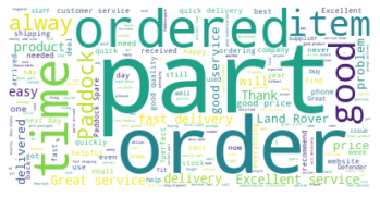
Now we’ve got the text preprocessed, we can create a basic word cloud. By instantiating WordCloud and then appending generate(text), we can pass in our big list of words and WordCloud will calculate the word frequencies, and determine the sizes, and colours of each of the words shown based on their frequencies within the text. The other bits of Matplotlib code turn off the axes and ticks to make the word cloud look a bit neater.
wordcloud = WordCloud(background_color="white").generate(text)
plt.imshow(wordcloud, interpolation='bilinear')
plt.axis("off")
plt.margins(x=0, y=0)
plt.show()
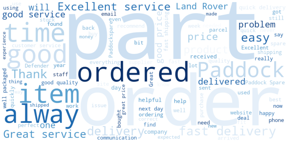
Customise the word cloud style
By default, the word clouds produced by WordCloud are very small. You can define their size using a combination of width and height arguments to WordCloud(), and by manually setting the size using figsize. You may want to tweak the number of words shown using max_words and set a maximum font size using max_font_size to get the look you want.
The background colour can be set using background_color. To change the colours used you can pass in any of the
Matplotlib colormap values. There’s a full list of these in the colormap section of the Matplotlib documentation
.
wordcloud = WordCloud(background_color="white",
                      max_words=100,
                      max_font_size=300,
                      width=1024,
                      height=500,
                      colormap="Blues"
                     ).generate(text)

plt.figure(figsize=(20,20))
plt.imshow(wordcloud, interpolation='bilinear')
plt.axis("off")
plt.margins(x=0, y=0)
plt.show()
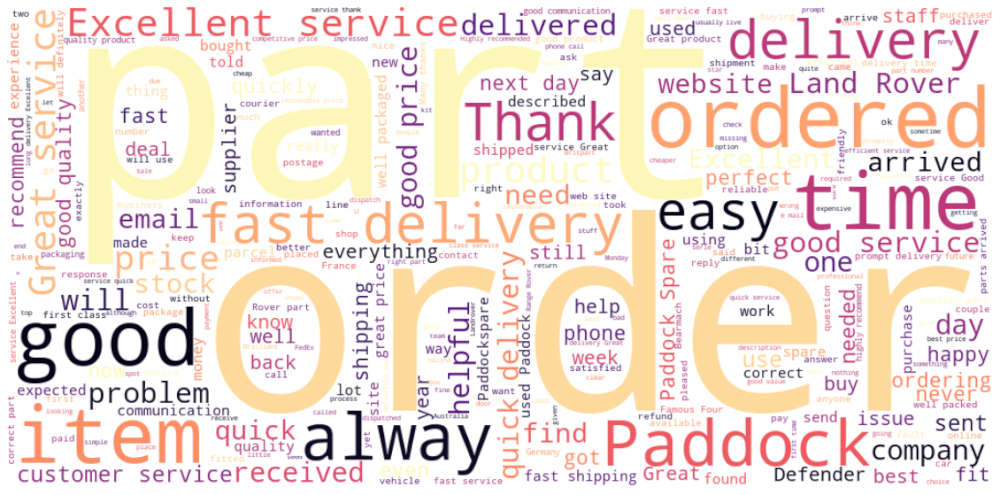
Saving the word cloud as a file
Finally, we can save our word cloud as an image file using the savefig() function from Matplotlib. This needs to go before plt.show() is called. Your word cloud is then saved to a file with your specified dimensions, so you can use it in your report or presentation.
wordcloud = WordCloud(background_color="white",
                      max_words=300,
                      width=1024,
                      height=500,
                      colormap="magma"
                     ).generate(text)

plt.figure(figsize=(20,20))
plt.imshow(wordcloud, interpolation='bilinear')
plt.axis("off")
plt.margins(x=0, y=0)
plt.savefig("cloud.png", format="png")
plt.show()
Matt Clarke, Sunday, March 07, 2021


Other posts you might like

How to use the Pandas truncate() function
Have you ever needed to chop the top or bottom off a Pandas dataframe, or extract a specific section from the middle? If so, there’s a Pandas function called truncate()...

How to use Spacy for noun phrase extraction
Noun phrase extraction is a Natural Language Processing technique that can be used to identify and extract noun phrases from text. Noun phrases are phrases that function grammatically as nouns...
