How to write better code using DRY and Do One Thing
Learn how to use the Don’t Repeat Yourself and Do One Thing techniques to help you create Python code that is easier to read, understand, and maintain.

DRY, or Don’t Repeat Yourself, and the “Do One Thing” methodology are designed to help software engineers and data scientists create better functions. Code that isn’t written using DRY tends to include repetition, often because the developer has cut and pasted a chunk and swapped out some values.
While this works fine, and is the norm in most Jupyter notebook code, it can introduce errors. It also means you need to make edits in many parts of the code, if you decide to change the way a particular repeated part of the code should function.
DRY aims to resolve this by creating functions that can be reused throughout your work. If you need to edit or improve the code, you can do it in a single place. Along with adherence to Python style guidelines, DRY can make your code much easier to read, especially if you name your functions sensibly to describe what they do.
Do One Thing
Another popular methodology in software engineering is called Do One Thing. As the name suggests, the theory is that functions should serve a single purpose, not do several things. While DRY is the norm in most projects, Do One Thing isn’t always used, but is a best practice worth learning.
Do One Thing makes the functions even easier to read, use, test, and debug, since they only do one thing. In addition, since they perform a single task, you can often re-use the same code in many parts of your project, or use them across projects. When combined with DRY, Do One Thing helps you generate much better Python functions. The minor downside is that you will need to write more functions, but at least you can re-use them.
Load the data
To show the DRY and Do One Thing approaches in action, we’ll do things the normal way, then apply DRY, then add in Do One Thing. I’m using the Online Retail II dataset from the UCI Machine Learning Repository. I’ve made some tweaks to this to adjust the column names and have calculated the line_price value for each row myself.
import pandas as pd
import datetime as dt
import seaborn as sns
import matplotlib.pyplot as plt

sns.set(rc={'figure.figsize':(15, 6)})
%config InlineBackend.figure_format = 'retina'
sns.set_context('notebook')

df = pd.read_csv('online-retail.csv', parse_dates=['order_date'])
df.head()
| order_id | sku | description | quantity | order_date | item_price | customer_id | country | line_price | |
|---|---|---|---|---|---|---|---|---|---|
| 0 | 489434 | 85048 | 15CM CHRISTMAS GLASS BALL 20 LIGHTS | 12 | 2009-12-01 07:45:00 | 6.95 | 13085.0 | United Kingdom | 83.4 |
| 1 | 489434 | 79323P | PINK CHERRY LIGHTS | 12 | 2009-12-01 07:45:00 | 6.75 | 13085.0 | United Kingdom | 81.0 |
| 2 | 489434 | 79323W | WHITE CHERRY LIGHTS | 12 | 2009-12-01 07:45:00 | 6.75 | 13085.0 | United Kingdom | 81.0 |
| 3 | 489434 | 22041 | RECORD FRAME 7" SINGLE SIZE | 48 | 2009-12-01 07:45:00 | 2.10 | 13085.0 | United Kingdom | 100.8 |
| 4 | 489434 | 21232 | STRAWBERRY CERAMIC TRINKET BOX | 24 | 2009-12-01 07:45:00 | 1.25 | 13085.0 | United Kingdom | 30.0 |
The old way
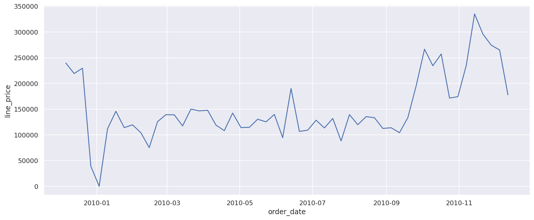
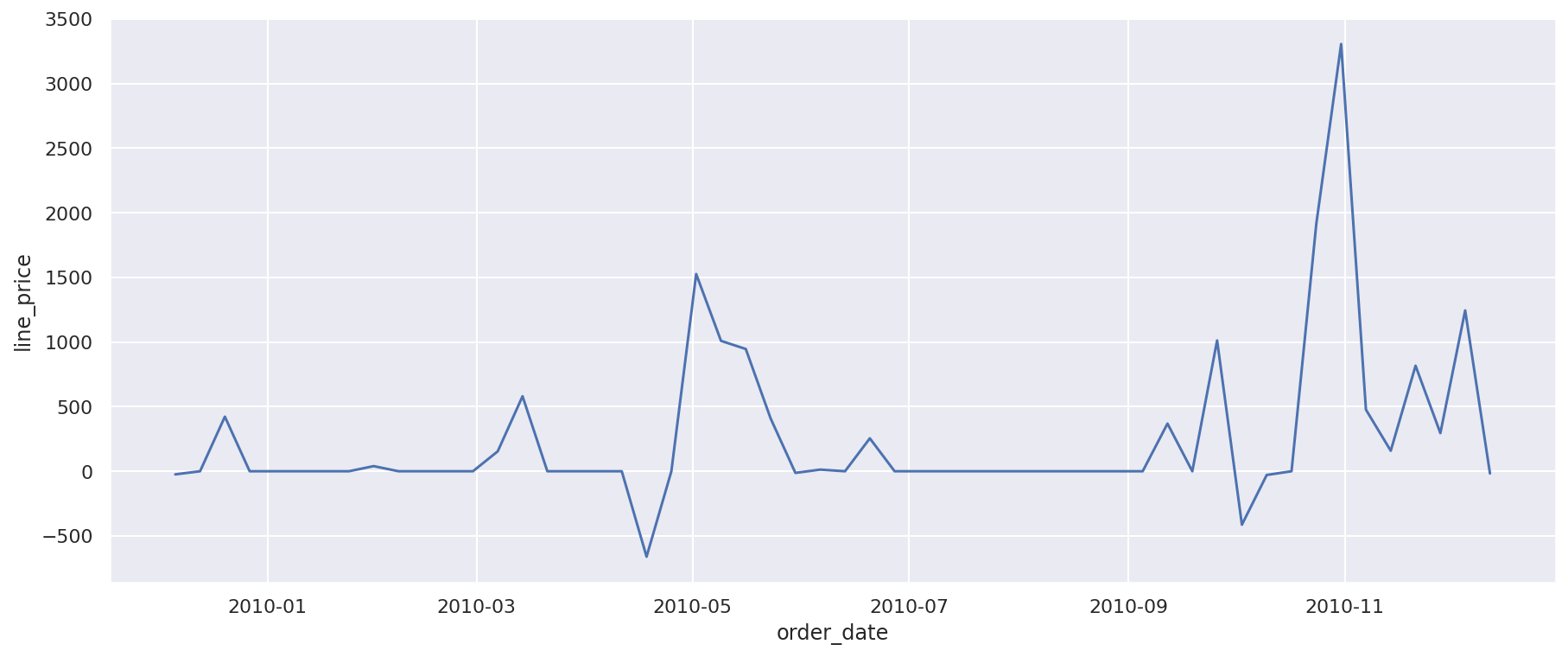
Let’s say we want to plot the weekly sales for a given country on a separate line plot using Seaborn. To do this we need to group the data on the country column, set the index to the order_date, resample the data to weekly, calculate the sum of the line_price column for the period, convert the data to a Pandas dataframe and then reset the index. Once we’ve got the data, we then need to pass the order_date column to Seaborn to use on the x axis and the line_price for the y axis, along with the dataframe created. Then we repeat the code for each country we want to plot.
df_weekly = df[df['country']=='United Kingdom'].set_index('order_date').\
resample('W')["line_price"].sum().to_frame().reset_index()

line = sns.lineplot(x='order_date',
                    y='line_price',
                    data=df_weekly)
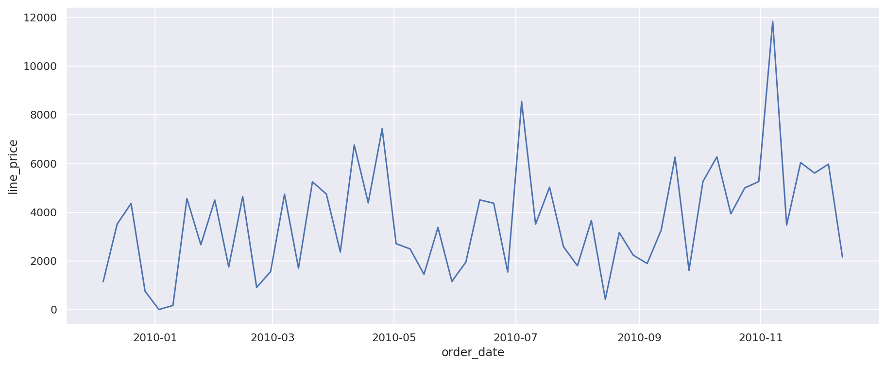
df_weekly = df[df['country']=='Germany'].set_index('order_date').\
resample('W')["line_price"].sum().to_frame().reset_index()

line = sns.lineplot(x='order_date',
                    y='line_price',
                    data=df_weekly)
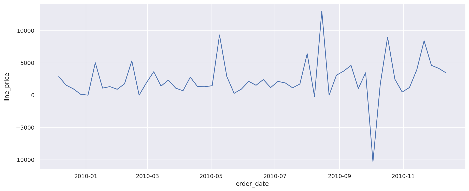
df_weekly = df[df['country']=='France'].set_index('order_date').\
resample('W')["line_price"].sum().to_frame().reset_index()

line = sns.lineplot(x='order_date',
                    y='line_price',
                    data=df_weekly)
Creating a DRY function
To make this a bit neater, we can use the DRY methodology to create a single function that takes the Pandas dataframe and a string containing a country name, and use it to create the Seaborn lineplot showing weekly sales for that region. All it takes is adding plot_sales_by_country(df, 'Spain'), or similar, for each country and we’ll generate a plot.
def plot_sales_by_country(df, country):
    """Plot total sales by country using Pandas and Seaborn.

    Parameters
    ----------
    df : Dataframe
        Online Retail II dataframe

    country : str
        Country name, i.e. United Kingdom

    Returns
    -------
        Prints Seaborn lineplot of sales for country

    """

    df_weekly = df[df['country']==country].set_index('order_date').\
    resample('W')["line_price"].sum().to_frame().reset_index()

    line = sns.lineplot(x='order_date',
                        y='line_price',
                        data=df_weekly)
plot_sales_by_country(df, 'Spain')
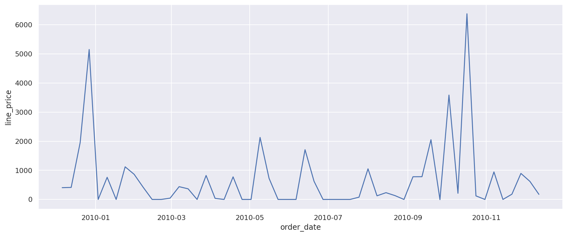
plot_sales_by_country(df, 'Italy')
Using DRY with Do One Thing
If we look at the plot_sales_by_country() function above, we can see that there are a number of things we can do to split out the actions it performs. There are two main parts to it. The first section takes our original dataframe, groups it by country, resamples the data to weekly, and then creates a Pandas dataframe containing the weekly sales metrics. The second section takes the data from the dataframe above and produces a lineplot() using Seaborn.
Let’s split the function out into two separate functions, one to calculate the weekly sales for the country, and another to plot the data. We’ll then be able to use one function to fetch the raw data, and the other to create the time series plot.
def get_sales_by_country(df, country, period='W'):
    """Return sales by country for a given periodicity.

    Parameters
    ----------
    df : Dataframe
        Online Retail II dataframe

    country : str
        Country name, i.e. United Kingdom

    period: str
        Pandas period identifier, i.e. D, W, M, Q, or Y

    Returns
    -------
        Pandas dataframe containing the specified data.

    """

    df_grouped = df[df['country']==country].set_index('order_date')\
    .resample(period)["line_price"].sum().to_frame().reset_index()

    return df_grouped
def plot_time_series_data(df, x_column='order_date', y_column='line_price'):
    """Create a time series line plot from the provided dataframe.

    Parameters
    ----------
    df : Dataframe
        Dataframe containing x and y columns from get_sales_by_country()

    x_column : str, optional
        Name of X column. Default 'order_date'.

    y_column : str, optional
        Name of y column. Default 'line_price'.

    Returns
    -------
        Seaborn line plot of time series data.

    """

    plot = sns.lineplot(x=x_column, y=y_column, data=df)
    return plot
df_monthly = get_sales_by_country(df, 'United Kingdom', 'M')
plot = plot_time_series_data(df_monthly)
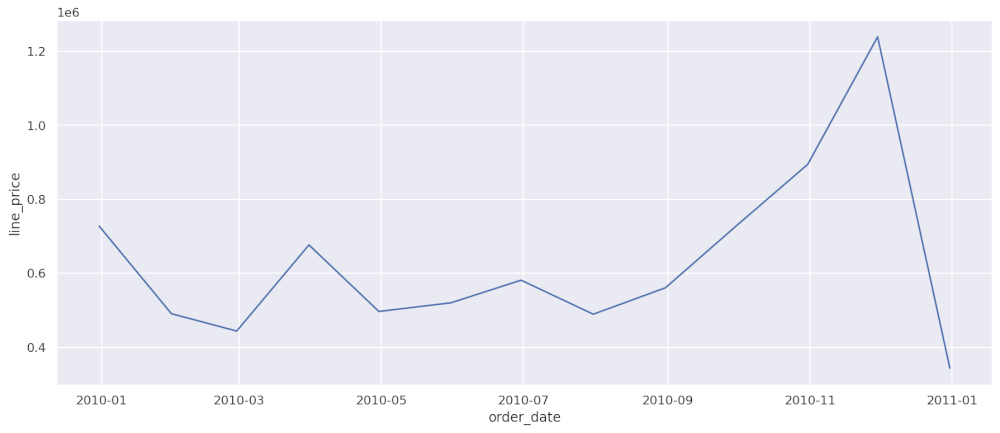
Further improvements
Obviously, there’s far more we could do that just this very basic example! We’ve already improved the code by allowing it to let the user specify different periods, such as weekly, monthly, or quarterly. However, we could also modify the function to allow the user to specify which metric, or metrics, were plotted. Hopefully, this very basic example should be enough to help you write cleaner, more maintainable code.
Matt Clarke, Monday, March 08, 2021


Other posts you might like

How to use the Pandas truncate() function
Have you ever needed to chop the top or bottom off a Pandas dataframe, or extract a specific section from the middle? If so, there’s a Pandas function called truncate()...

How to use Spacy for noun phrase extraction
Noun phrase extraction is a Natural Language Processing technique that can be used to identify and extract noun phrases from text. Noun phrases are phrases that function grammatically as nouns...
