How to create Google Search Console time series forecasts using Neural Prophet
Learn how to use the Neural Prophet model and EcommerceTools to create time series forecasts of your Google Search Console search performance data.

Time series forecasting uses machine learning to predict future values of time series data. In this project we’ll be using the Neural Prophet model to predict future values of Google Search Console search performance data.
Neural Prophet is a time series forecasting model, powered by PyTorch, that uses a neural network to predict future values of time series data. It’s a great way to use machine learning to predict future values of time series data.
It was inspired by the excellent Facebook Prophet model, but uses Gradient Descent for optimisation, allows autocorrelation via AR-Net, and lets you use lagged regressors via a separate Feed Forward Neural Network. It sounds pretty complicated, but it’s actually not that hard to use, and gives pretty good results.
Install the packages
To create our time series forecast of Google Search Console performance data we’ll require the Pandas library and two other Python packages. To fetch your Google Search Console data using the API we’ll be using my EcommerceTools Python package. This lets you query GSC using Python, and do a whole load of other useful things for ecommerce, marketing, and SEO projects.
For the time series forecasting bit we’ll be using the Neural Prophet package. This was inspired by Facebook’s excellent Prophet time series forecasting model, but has a few extra features. It’s very easy to use, but it uses a PyTorch backend, so your Python environment will need to have this set up. I’m using the NVIDIA Data Science Stack Docker container, and Neural Prophet and PyTorch can run on it out of the box.
!pip3 install neuralprophet[live]
!pip3 install ecommercetools
Load the packages
Once you’ve installed Neural Prophet and EcommerceTools, import the packages below. We’ll be using the seo module from EcommerceTools, the NeuralProphet module from Neural Prophet, and the set_random_seed feature to allow reproducible results between runs of the model.
import pandas as pd
from ecommercetools import seo
from neuralprophet import NeuralProphet
from neuralprophet import set_random_seed
set_random_seed(0)
Configure your Google Search Console API connection
Next, you’ll need to configure some variables to pass to EcommerceTools, so it can authenticate against your Google Search Console API account. This is done using a Google Cloud Service Account via a client secrets JSON keyfile.
Create a client secrets JSON keyfile, define the URL you want to query, and set the start date and end date. This site is still quite new, so I don’t have very much data to play with, but I would advise that you set the longest duration you can to obtain the best forecast.
key = "pds-client-secrets.json"
site_url = "sc-domain:practicaldatascience.co.uk"
start_date = "2021-03-01"
end_date = "2021-10-31"
Fetch your Google Search Console data
Now we need to create a “payload” dictionary that EcommerceTools can pass to the Google Search Console API. This needs to include the startDate, endDate, and a list of dimensions that must include the date, since we want our data grouped by day for the model.
payload = {
    'startDate': start_date,
    'endDate': end_date,
    'dimensions': ["date"],
}
Once you’ve created your payload dictionary, you can pass it to the seo.query_google_search_console() function along with the key variable holding the path to your client secrets JSON keyfile, and the site_url variable holding the URL of the domain you want to query. The function returns a Pandas dataframe.
If you print the head() of the dataframe you’ll see that it contains clicks, impressions, ctr, and position. You can forecast any of these metrics using the model, simply by modifying the code below.
df = seo.query_google_search_console(key, site_url, payload)
df.sort_values(by='date', ascending=False).head()
| date | clicks | impressions | ctr | position | |
|---|---|---|---|---|---|
| 244 | 2021-10-31 | 458 | 18762 | 2.44 | 29.70 |
| 243 | 2021-10-30 | 355 | 17206 | 2.06 | 30.91 |
| 242 | 2021-10-29 | 650 | 25269 | 2.57 | 25.83 |
| 241 | 2021-10-28 | 819 | 29741 | 2.75 | 23.89 |
| 240 | 2021-10-27 | 864 | 31293 | 2.76 | 23.77 |
Reformat the data for the Neural Prophet model
Like the Facebook Prophet model, Neural Prophet also requires that you reformat the input dataframe you pass to the model when training the time series forecast model. This needs to have two columns: ds holding the date, and y containing the target variable you want the model to forecast.
We can use the Pandas rename() function to take our original df dataframe and rename the dataframe columns accordingly. We’ll initially forecast clicks by renaming the clicks column y and then saving the output dataframe to data to avoid overwriting the original.
data = df.rename(columns={'date': 'ds', 'clicks': 'y'})[['ds', 'y']]
data.head()
| ds | y | |
|---|---|---|
| 0 | 2021-03-01 | 0 |
| 1 | 2021-03-02 | 0 |
| 2 | 2021-03-03 | 0 |
| 3 | 2021-03-04 | 0 |
| 4 | 2021-03-05 | 0 |
Create the Neural Prophet forecasting model
Neural Prophet includes various options that you can pass to the model to generate more accurate time series forecasts. Since my site doesn’t really have weekly or monthly seasonality, but traffic does vary during the week, I’ve set daily_seasonality to True. I’ve then used fit() to build the fit the model on the data using daily data frequency to match what we exported from Google Search Console. This model will run pretty quickly on a GPU.
model = NeuralProphet(daily_seasonality=True)
metrics = model.fit(data, freq="D")
INFO - (NP.utils.set_auto_seasonalities) - Disabling yearly seasonality. Run NeuralProphet with yearly_seasonality=True to override this.
INFO - (NP.config.set_auto_batch_epoch) - Auto-set batch_size to 16
INFO - (NP.config.set_auto_batch_epoch) - Auto-set epochs to 256


HBox(children=(HTML(value=''), FloatProgress(value=0.0, max=220.0), HTML(value='')))


INFO - (NP.utils_torch.lr_range_test) - lr-range-test results: steep: 1.00E-01, min: 8.02E-01
INFO - (NP.utils_torch.lr_range_test) - learning rate range test selected lr: 4.01E-01
Epoch[256/256]: 100%|██████████| 256/256 [00:06<00:00, 41.93it/s, SmoothL1Loss=0.00432, MAE=56.4, MSE=4.99e+3, RegLoss=0]
Create a future dataframe
Now the model is built, we need to create another dataframe containing the dates for the future period. You can do this using the make_future_dataframe() function. I’ve set this to a duration of 365 days, so we forecast one year into the future. You can view the output of the future dataframe by printing the head().
future = model.make_future_dataframe(data, periods=365, n_historic_predictions=True)
future.head()
| ds | y | t | y_scaled | |
|---|---|---|---|---|
| 0 | 2021-03-01 | 0 | 0.000000 | 0.0 |
| 1 | 2021-03-02 | 0 | 0.004098 | 0.0 |
| 2 | 2021-03-03 | 0 | 0.008197 | 0.0 |
| 3 | 2021-03-04 | 0 | 0.012295 | 0.0 |
| 4 | 2021-03-05 | 0 | 0.016393 | 0.0 |
Create the time series forecast
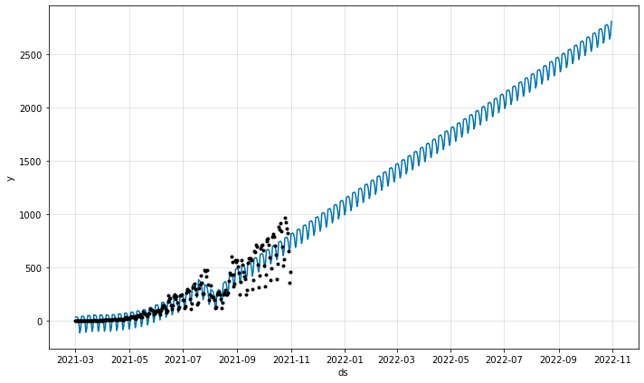
Now we’ll create a forecast. To do this we simply pass the future dataframe to the predict() function. We can then pass the forecast output to the plot() function to view the time series forecast itself. The blue line represents the model’s forecast for the clicks variable we passed to the model. The black dots represent the actual values in the previous period.
As you can see from my data, there’s a decent upward trend in the clicks, as well as an odd dip during August, which seemed to coincide with a Google algorithm change, and then a subsequent reversal of the impact a month or so later.
forecast = model.predict(future)
model.plot(forecast)

Examine the forecast
To examine the actual values that have been forecast, you can print the output of the forecast dataframe. The dataframe gives you the date, the actual value recorded y, plus various other components from the time series, including the trend, seasonality, and forecast value in yhat1.
forecast.head()
| ds | y | yhat1 | residual1 | trend | season_weekly | season_daily | |
|---|---|---|---|---|---|---|---|
| 0 | 2021-03-01 | 0 | 34.964188 | 34.9642 | -92.075294 | 52.409801 | 74.629684 |
| 1 | 2021-03-02 | 0 | 32.497509 | 32.4975 | -91.105042 | 48.972870 | 74.629684 |
| 2 | 2021-03-03 | 0 | 34.239559 | 34.2396 | -90.134789 | 49.744667 | 74.629684 |
| 3 | 2021-03-04 | 0 | 19.703564 | 19.7036 | -89.164528 | 34.238403 | 74.629684 |
| 4 | 2021-03-05 | 0 | -28.811146 | -28.8111 | -88.194275 | -15.246559 | 74.629684 |
forecast.tail()
| ds | y | yhat1 | residual1 | trend | season_weekly | season_daily | |
|---|---|---|---|---|---|---|---|
| 605 | 2022-10-27 | None | 2765.863525 | NaN | 2656.995361 | 34.238403 | 74.629684 |
| 606 | 2022-10-28 | None | 2721.852539 | NaN | 2662.469482 | -15.246559 | 74.629684 |
| 607 | 2022-10-29 | None | 2640.049805 | NaN | 2667.943115 | -102.522743 | 74.629684 |
| 608 | 2022-10-30 | None | 2680.449951 | NaN | 2673.416748 | -67.596420 | 74.629684 |
| 609 | 2022-10-31 | None | 2805.930176 | NaN | 2678.890625 | 52.409801 | 74.629684 |
Plot the forecast components
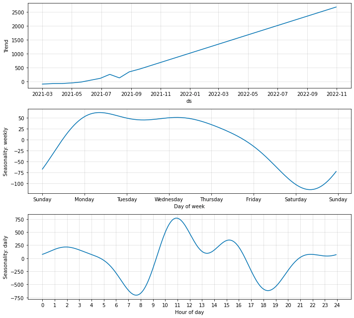
The time series decomposition technique can be used to extract the underlying components from within your time series. Neural Prophet makes time series decomposition very easy. You simply pass the forecast dataframe to the plot_components() function and it will give you a breakdown of each component.
As you can see, the trend component is growing steadily, apart from the odd Google algorithm related blip back in August. The weekly seasonality element shows that the site is busiest on a Monday and quietest on a Saturday, but it looks like lots of data scientists spending their Sunday relaxing by reading the website. The daily seasonality component shows that the peak hours are mid morning, and during normal office hours, with the commute hours being the quietest.
components = model.plot_components(forecast)
Matt Clarke, Friday, November 05, 2021


Other posts you might like

How to tune a LightGBMClassifier model with Optuna
The LightGBM model is a gradient boosting framework that uses tree-based learning algorithms, much like the popular XGBoost model. LightGBM supports both classification and regression tasks, and is known for...

How to create a customer retention model with XGBoost
Although all business know the importance of retaining customers, few companies are actually able to measure customer retention accurately, and fewer still can predict which ones will churn or be...
