How to avoid model overfitting with early stopping rounds
Overfitting reduces model performance. Here's how you can avoid it using the XGBoost early stopping rounds feature.

One issue with the more sophisticated algorithms, such as Extreme Gradient Boosting, is that they can overfit to the data. This basically means that the model picks up the idiosyncrasies in the data and follows it too closely, causing it to work well on the training data but fail to generalise when given unseen test data.
When these models are being trained they fit to the data dozens and dozens of times. What can happen is that, after a while, model performance stops improving and the accuracy or error rate actually starts to deteriorate as the model overfits.
However, there’s a useful parameter in XGBoost that allows you to reduce overfitting - it’s called early_stopping_rounds. The early stopping rounds parameter takes an integer value which tells the algorithm when to stop if there’s no further improvement in the evaluation metric. It can prevent overfitting and improve your model’s performance. Here’s a basic guide to how to use it.
Load the packages
In this simple example we’ll need only a handful of packages, that you probably already have installed. We’ll be using Pandas for data manipulation, Matplotlib for creating plots, the XGBClassifer from XGBoost, and the train_test_split and accuracy_score packages from sklearn.
import pandas as pd
import matplotlib.pyplot as plt
from xgboost import XGBClassifier
from sklearn.model_selection import train_test_split
from sklearn.metrics import accuracy_score
%config InlineBackend.figure_format = 'retina'
sns.set_context('notebook')
sns.set(rc={'figure.figsize':(15, 6)})
pd.set_option('max_columns', 6)
Load the data
You can load any data set you like. I’ve used a contractual churn model dataset as it only requires minor effort to prepare it for use in the model. Load up your data and display the first few lines using head().
df = pd.read_csv('train.csv')
df.head()
| state | account_length | area_code | churn | |
|---|---|---|---|---|
| 0 | OH | 107 | area_code_415 | no |
| 1 | NJ | 137 | area_code_415 | no |
| 2 | OH | 84 | area_code_408 | no |
| 3 | OK | 75 | area_code_415 | no |
| 4 | MA | 121 | area_code_510 | no |
Preprocess your data
This data needs some very simple preprocessing before we can use it. The churn column is current a boolean value, so we need to binarise that. We can also do a quick-and-dirty one-hot encoding of the other categorical values in here and it will be ready to use.
df['churn'] = np.where(df['churn'].str.contains('yes'), 1, 0)
df = pd.get_dummies(df)
Create the training and test data
We’ll assign all of the values in our dataframe to X, with the exception of the target churn parameter, which we’ll drop. The churn column is assigned to y, then we’ll pass these values to train_test_split() and get back our test and train datasets.
X = df.drop(columns=['churn'])
y = df['churn']
X_train, X_test, y_train, y_test = train_test_split(X, y,
                                                    test_size=0.3,
                                                    stratify=y,
                                                    random_state=0)
Fit a baseline model
To see what we’re starting with, we’ll fit a very quick baseline model using XGBClassifier on its default settings. This gives us an accuracy score on our churn prediction model of 96.24%. There’s a possibility that as the model goes through additional epochs, that the accuracy drops, so we’ll check that in our next step.
model = XGBClassifier()
model.fit(X_train, y_train)
y_preds = model.predict(X_test)
print('Accuracy:', round(accuracy_score(y_test, y_preds) * 100,2),'%')
Accuracy: 96.24 %
Fit the same model and show errors
Next, we’ll refit the exact same model, but pass in a few extra arguments to the fit() function. The eval_metric argument is set to error and will record the error rate on each epoch when comparing the training data to the test data, as defined by the eval_set argument. The verbose flag is set to True so we can see the errors generated on each epoch.
model = XGBClassifier()

model.fit(X_train,
          y_train,
          eval_metric="error",
          eval_set=[(X_test, y_test)],
          verbose=True)
[0]    validation_0-error:0.06039
[1]    validation_0-error:0.05255
[2]    validation_0-error:0.04863
[3]    validation_0-error:0.04392
[4]    validation_0-error:0.04078
[5]    validation_0-error:0.04157
[6]    validation_0-error:0.04000
[7]    validation_0-error:0.04078
[8]    validation_0-error:0.03686
[9]    validation_0-error:0.03686
[10]    validation_0-error:0.03608
[11]    validation_0-error:0.03372
[12]    validation_0-error:0.03372
[13]    validation_0-error:0.03765
[14]    validation_0-error:0.03608
[15]    validation_0-error:0.03529
[16]    validation_0-error:0.03765
[17]    validation_0-error:0.03686
[18]    validation_0-error:0.03686
[19]    validation_0-error:0.03529
[20]    validation_0-error:0.03686
[21]    validation_0-error:0.03765
[22]    validation_0-error:0.03608
[23]    validation_0-error:0.03843
[24]    validation_0-error:0.03608
[25]    validation_0-error:0.03529
[26]    validation_0-error:0.03529
[27]    validation_0-error:0.03608
[28]    validation_0-error:0.03686
[29]    validation_0-error:0.03843
[30]    validation_0-error:0.03922
[31]    validation_0-error:0.03765
[32]    validation_0-error:0.03922
[33]    validation_0-error:0.03922
[34]    validation_0-error:0.03843
[35]    validation_0-error:0.03843
[36]    validation_0-error:0.03608
[37]    validation_0-error:0.03765
[38]    validation_0-error:0.03843
[39]    validation_0-error:0.03765
[40]    validation_0-error:0.03765
[41]    validation_0-error:0.03765
[42]    validation_0-error:0.03765
[43]    validation_0-error:0.03843
[44]    validation_0-error:0.03765
[45]    validation_0-error:0.03451
[46]    validation_0-error:0.03529
[47]    validation_0-error:0.03529
[48]    validation_0-error:0.03529
[49]    validation_0-error:0.03765
[50]    validation_0-error:0.03765
[51]    validation_0-error:0.03922
[52]    validation_0-error:0.04000
[53]    validation_0-error:0.04000
[54]    validation_0-error:0.04078
[55]    validation_0-error:0.04078
[56]    validation_0-error:0.03922
[57]    validation_0-error:0.03843
[58]    validation_0-error:0.03843
[59]    validation_0-error:0.03843
[60]    validation_0-error:0.03686
[61]    validation_0-error:0.03922
[62]    validation_0-error:0.03843
[63]    validation_0-error:0.03922
[64]    validation_0-error:0.03765
[65]    validation_0-error:0.03843
[66]    validation_0-error:0.03765
[67]    validation_0-error:0.03686
[68]    validation_0-error:0.03608
[69]    validation_0-error:0.03686
[70]    validation_0-error:0.03686
[71]    validation_0-error:0.03608
[72]    validation_0-error:0.03608
[73]    validation_0-error:0.03608
[74]    validation_0-error:0.03765
[75]    validation_0-error:0.03843
[76]    validation_0-error:0.03765
[77]    validation_0-error:0.03843
[78]    validation_0-error:0.03843
[79]    validation_0-error:0.03765
[80]    validation_0-error:0.03922
[81]    validation_0-error:0.03922
[82]    validation_0-error:0.03922
[83]    validation_0-error:0.03922
[84]    validation_0-error:0.03843
[85]    validation_0-error:0.03686
[86]    validation_0-error:0.03686
[87]    validation_0-error:0.03686
[88]    validation_0-error:0.03686
[89]    validation_0-error:0.03765
[90]    validation_0-error:0.03608
[91]    validation_0-error:0.03686
[92]    validation_0-error:0.03686
[93]    validation_0-error:0.03686
[94]    validation_0-error:0.03686
[95]    validation_0-error:0.03686
[96]    validation_0-error:0.03686
[97]    validation_0-error:0.03686
[98]    validation_0-error:0.03686
[99]    validation_0-error:0.03765


XGBClassifier(base_score=0.5, booster='gbtree', colsample_bylevel=1,
              colsample_bynode=1, colsample_bytree=1, gamma=0, gpu_id=-1,
              importance_type='gain', interaction_constraints='',
              learning_rate=0.300000012, max_delta_step=0, max_depth=6,
              min_child_weight=1, missing=nan, monotone_constraints='()',
              n_estimators=100, n_jobs=0, num_parallel_tree=1, random_state=0,
              reg_alpha=0, reg_lambda=1, scale_pos_weight=1, subsample=1,
              tree_method='exact', validate_parameters=1, verbosity=None)
Obviously, we get exactly the same accuracy score as we’ve not changed our model. However, if you examine the numbers in the output above, you’ll notice that we start with an error of 0.06039 on the first epoch, which falls to 0.03372 by epoch 11. However, subsequent epochs see the error increase, as the model is overfitting to the data. It’s not a massive increase on this dataset, but it can be on others.
y_preds = model.predict(X_test)
print('Accuracy:', round(accuracy_score(y_test, y_preds) * 100,2),'%')
Accuracy: 96.24 %
Create a model learning curve
We can plot the drop off in the error rate, and its subsequent increase through epochs, by capturing the output of the model errors using the result() function. First, we’ll re-run the above model once again and store the results for the train and test data in a dictionary called results.
eval_set = [(X_train, y_train), (X_test, y_test)]
model.fit(X_train,
          y_train,
          eval_metric="error",
          eval_set=eval_set,
          verbose=False)
results = model.evals_result()
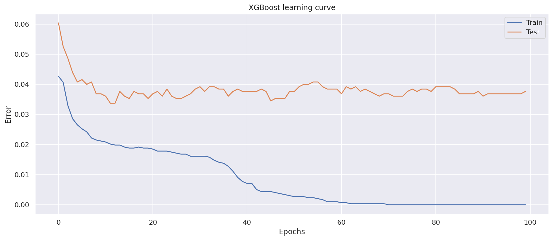
Now we can use Matplotlib to plot our learning curve. This shows the error rate for the train and test datasets at each epoch. You can see that the low point on the orange Test line represents that minimum error point we spotted in the data above, and you can see that it goes up slightly in subsequent epochs. That indicates the point at which the model should stop to maximise its performance.
epochs = len(results['validation_0']['error'])
x_axis = range(0, epochs)

fig, ax = plt.subplots()
ax.plot(x_axis, results['validation_0']['error'], label='Train')
ax.plot(x_axis, results['validation_1']['error'], label='Test')
ax.legend()
plt.xlabel('Epochs')
plt.ylabel('Error')
plt.title('XGBoost learning curve')
plt.show()
Using early stopping rounds
Finally, we can run this again and pass in an extra argument called early_stopping_rounds to the fit() function. This tells the model to stop if the score hasn’t improved after the defined number of epochs or rounds. Therefore, setting this to 5 results in our best iteration being the one with our minimum error score of 0.03372.
model = XGBClassifier()

model.fit(X_train,
          y_train,
          eval_metric="error",
          eval_set=[(X_test, y_test)],
          early_stopping_rounds=5,
          verbose=True)

y_preds = model.predict(X_test)
[0]    validation_0-error:0.06039
Will train until validation_0-error hasn't improved in 5 rounds.
[1]    validation_0-error:0.05255
[2]    validation_0-error:0.04863
[3]    validation_0-error:0.04392
[4]    validation_0-error:0.04078
[5]    validation_0-error:0.04157
[6]    validation_0-error:0.04000
[7]    validation_0-error:0.04078
[8]    validation_0-error:0.03686
[9]    validation_0-error:0.03686
[10]    validation_0-error:0.03608
[11]    validation_0-error:0.03372
[12]    validation_0-error:0.03372
[13]    validation_0-error:0.03765
[14]    validation_0-error:0.03608
[15]    validation_0-error:0.03529
[16]    validation_0-error:0.03765
Stopping. Best iteration:
[11]    validation_0-error:0.03372
If you re-run the accuracy function, you’ll see performance has improved slightly from the 96.24% score of the baseline model, to a score of 96.63% when we apply early stopping rounds. This has reduced some minor overfitting on our model and given us a better score.
print('Accuracy:', round(accuracy_score(y_test, y_preds) * 100,2),'%')
Accuracy: 96.24 %
There are still further tweaks you can make from here. Often, adjusting the n_estimators and learning_rate in conjunction with early_stopping_rounds can get you further incremental improvements. They’re not that dramatic here, but every little helps, and they can really make a difference when your model is overfitting your data.
Matt Clarke, Saturday, August 14, 2021


Other posts you might like

How to tune a LightGBMClassifier model with Optuna
The LightGBM model is a gradient boosting framework that uses tree-based learning algorithms, much like the popular XGBoost model. LightGBM supports both classification and regression tasks, and is known for...

How to create a customer retention model with XGBoost
Although all business know the importance of retaining customers, few companies are actually able to measure customer retention accurately, and fewer still can predict which ones will churn or be...
