How to build the 'Hotdog , not Hotdog' image classifier
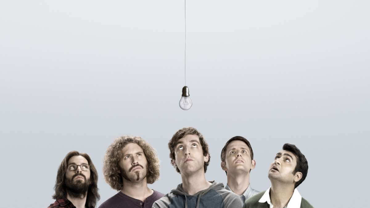
Learn how to classify images using Keras and TensorFlow by building the 'Hotdog, Not Hotdog' Convolutional Neural Net image classifier from Silicon Valley.
Convolutional Neural Networks or CNNs are one of the most widely used AI techniques for detecting complex features in data. They’re particularly good for image recognition, and are used in many autonomous robots, self-driving cars and object and facial recognition systems.
With the growth of applications like Tensorflow and packages such as Keras and PyTorch, not to mention crazily powerful CPUs and GPUs, it’s become much quicker and easier to create Convolutional Neural Nets and, today, a couple of hours’ coding can generate results that would have been considered world-class a few years ago.
In this example, we’re going to walk through the steps you need to follow to make a CNN that can classify images and explain a little about how they work in the process.
Creating your CNN
Obtaining an image classification dataset
Obviously, the first thing we’re going to need is an image classification dataset. This needs to include plenty of images of the things you’re aiming to classify with your model, and the image need to be labelled by placing them in separate directories based on their class. The technique used here works for pretty much any images, but I’m going with the a simple binary classification problem to determine whether a picture is of a “hotdog” or “not hotdog” using this wonderful dataset. You are free to apply this to any kind of images you wish to classify.
Fans of the data science themed TV series Silicon Valley will be aware that the same technology was used by Jian Yang in his Seefood AI app which was intended to be the “Shazam for food” but was capable only of detecting whether a food item was a hotdog or not a hotdog.
“Jian-Yang. Motherfuck. I gave you the ability to spin gold, and instead, you’ve spun pubic hair with shit in it, and gravel and corn…”
It turned out that Jian Yang’s app also happened to be great at detecting pictures of other, ahem, sausage-shaped objects, and it ended up being acquired by Periscope for $4 million. If you end up selling your version, please cut me a slice of the royalties! Perhaps I could buy a palapa?
If you’ve never done any image classification before, you’re probably wondering how on earth a Convolutional Neural Net is even capable of doing this. Well, although us humans see images in a visual way, images are actually just made up of tiny squares called pixels. Each one is a specific number of pixels wide and a specific number of pixels high, and each pixel is a different colour. The colour in each pixel is represented by a number from 0 to 255, so computers can essentially see them as a large matrix of numbers.
To massively oversimplify, the CNN takes the matrix from the input image and uses a feature detector (also called a kernel or filter) to produce a feature map or “convolved feature”.
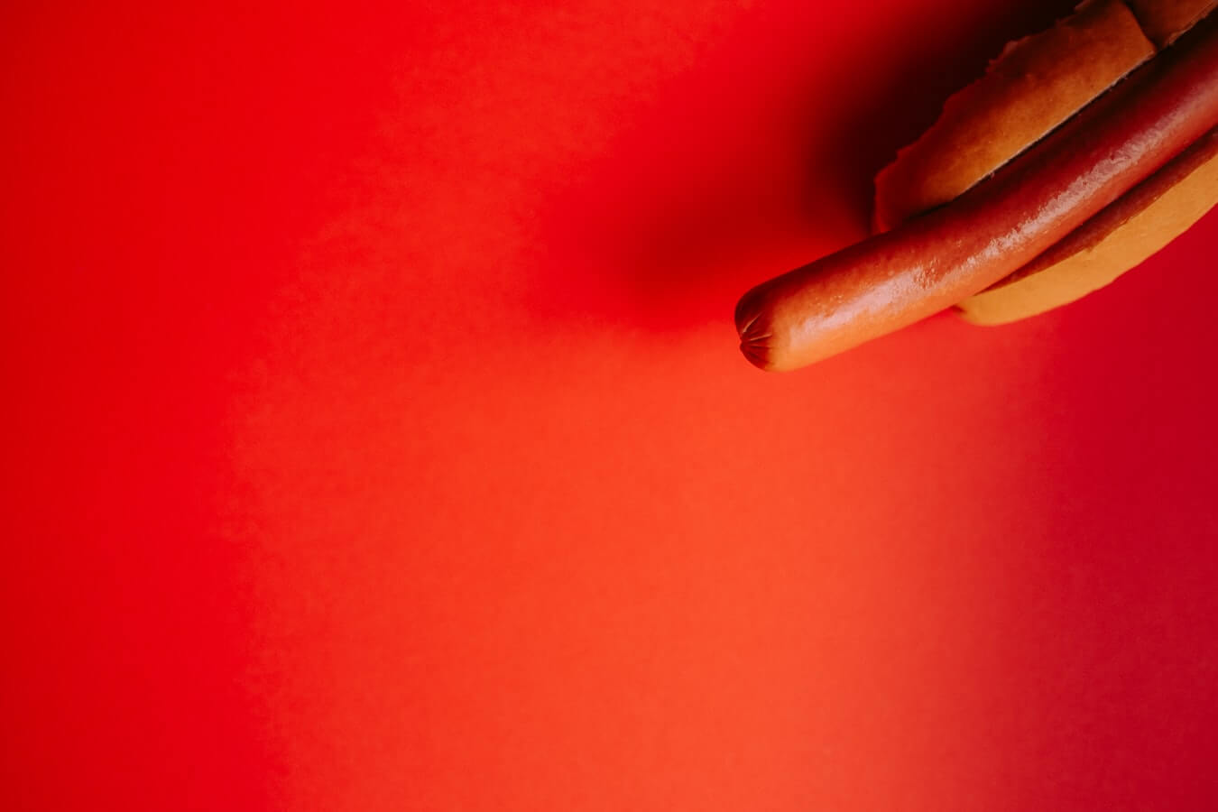 Hotdog. Annie Spratt, Unsplash.
Data augmentation
Once you found an interesting and labelled dataset of images to classify, the next step is to “augment” your data. Data augmentation is a useful step in image classification and does two main things: it gives you extra data to train with and it helps reduce overfitting. What happens in this step is that the images are tweaked to change their appearance slightly. Each image will be randomly rotated by varying degrees, moved left and right, scaled in and out, twisted or sheered, flipped in various orientations, zoomed in and out, and then normalised.
This creates loads of new images and makes the data more diverse and realistic. This allows your model to train on images that more closely resemble those its likely to encounter in the real world, so it generalises better and gives more accurate results when in production. Keras provides a useful class for image augmentation called ImageDataGenerator(), so we’ll first set this up with our desired parameters, then we’ll examine a sample image and see how it gets augmented.
import tensorflow as tf
from tensorflow import keras
from keras.preprocessing.image import ImageDataGenerator, array_to_img, img_to_array, load_img

datagen = ImageDataGenerator(
    rotation_range=40,
    width_shift_range=0.2,
    height_shift_range=0.2,
    rescale=1./255,
    shear_range=0.2,
    zoom_range=0.2,
    horizontal_flip=True,
    fill_mode='nearest'
)
Examining the augmented images
To visualise what happened in the above step, we’ll run the data augmentation process on a single image and look at the output to help understand what happens behind the scenes. We’ll load a random hotdog image and use the img_to_array() function to convert the image to a Numpy array and then run the Keras flow() function to examine how it gets augmented by the datagen we created above. We’ll store the augmented images in data/preview/hotdog/ and prefix the images with hotdog and create 30 different variations before stopping. As you’ll see in the image below, the directory gets filled with 30 new derivatives of the original image.
img = load_img('data/train/hotdog/4.jpg')
x = img_to_array(img)
x = x.reshape((1,) + x.shape)

i = 0
for batch in datagen.flow(x,
                          batch_size=1,
                          save_to_dir='data/preview/hotdog/',
                          save_prefix='hotdog',
                          save_format='jpg'):
    i += 1
    if i > 30:
        break
Load the training images
Next, we’ll load the augmented images from the training dataset into train_generator and validation_generator so they can be used by the model. We used the flow() function in the example above, but there’s also a more appropriate function called flow_from_directory() in Keras which can import all of the images in a directory, instead of loading a single one.
As the images in our training dataset folder are neatly stored with one class in each folder, we can pass the flow_from_directory() function the name of the directory data/train/ and it will find the included hotdog and nothotdog directories and load in the images. It finds 3000 source images in two classes in the train dataset and 644 images in two classes in the test dataset that we’ll use for validation.
train_generator = datagen.flow_from_directory(
    "data/train/",
    target_size=(300, 300),
    batch_size=128,
    class_mode="binary"
)
validation_generator = datagen.flow_from_directory(
    "data/test/",
    target_size=(300, 300),
    batch_size=128,
    class_mode="binary"
)
Create the convolutional neural network
Now that we’ve loaded our augmented images, we can move onto the exciting part - creating the model itself. There are a few types of model you can use for image classification, but convolutional neural networks are arguably the most commonly used.
Convolutional neural networks (also known as convnets or CNNs) are ideal for image classification tasks, but they can suffer from overfitting, where the model learns all there is to know to generate fantastic results on the training data but performs poorly on images it’s never seen before, picking up on small but irrelevant features that don’t actually help. The data augmentation step we used earlier really helps avoid overfitting, but there is another factor to consider when training convnets - entropic capacity.
Entropic capacity basically defines how much information your convnet is permitted to store and re-use. While you might think that the ability to memorise more data would be handy, the risk is that it will store irrelevant features that cause overfitting.
from keras.models import Sequential
from keras.layers import Conv2D, MaxPooling2D, Activation, Dropout, Flatten, Dense

model = tf.keras.models.Sequential()

model.add(tf.keras.layers.Conv2D(16, (3,3), activation='relu', input_shape=(300, 300, 3)))
model.add(tf.keras.layers.MaxPooling2D(2, 2))

model.add(tf.keras.layers.Conv2D(32, (3,3), activation='relu'))
model.add(tf.keras.layers.MaxPooling2D(2,2))

model.add(tf.keras.layers.Conv2D(64, (3,3), activation='relu'))
model.add(tf.keras.layers.MaxPooling2D(2,2))

model.add(tf.keras.layers.Conv2D(64, (3,3), activation='relu'))
model.add(tf.keras.layers.MaxPooling2D(2,2))

model.add(tf.keras.layers.Conv2D(64, (3,3), activation='relu'))
model.add(tf.keras.layers.MaxPooling2D(2,2))

model.add(tf.keras.layers.Flatten())
model.add(tf.keras.layers.Dense(512, activation='relu'))
model.add(tf.keras.layers.Dropout(0.5))
model.add(tf.keras.layers.Dense(1, activation='sigmoid'))
The Keras summary() function allows you to see all of the model parameters in a neat table. Tuning the parameters above and changing your model’s configuration can help you identify what works best and can give you further improvements in performance.
model.summary()
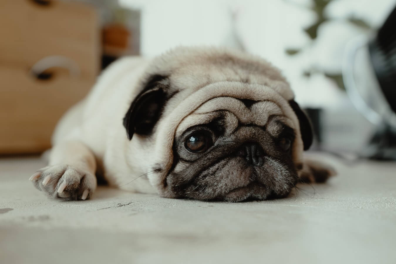 Not hotdog. JC Gellidon, Unsplash.
Compile model
from tensorflow.keras.optimizers import RMSprop

model.compile(loss='binary_crossentropy',
              optimizer=RMSprop(lr=0.001),
              metrics=['accuracy'])
Fit model
Next, it’s time to fit the model. The Keras documentation says you should use the fit_generator() function, but this is soon to be deprecated, so instead you can use fit() as this now supports generators. The time this takes to run will depend on the size of your images and dataset, the number of epochs and the batch size you use, the number of layers in your neural net, and the speed of your computer.
On my 4GHz Ryzen 3700X machine with 64GB of RAM each epoch takes about 16 seconds to run on a CPU. On a GPU, it will be over in a fraction of the time, but you will need to go through the pain of configuring CUDA and CuDNN and getting your Nvidia drivers working, which can be a painful experience.
As the verbose flag is set to 1, you get to watch the model’s accuracy improving as it works its way through the epochs. At the start, the model was no better than random guessing with just 50% accuracy, but it gets better every time, generating strong results by the end of training. You need to carefully set the steps_per_epoch and the number of epochs to calculate the number of batches. The number of batches is calculated by steps_per_epoch * epochs so 50 * 5 = 250, and if your input data runs out the model will stop.
history = model.fit(
    train_generator,
    steps_per_epoch=8,
    epochs=15,
    #validation_data=validation_generator,
    #validation_steps=8,
    verbose=1)

model.save_weights('weights.h5')
Examine predictions
Now that the model has run, let’s take a look at some predictions. The very vast majority are predicted correctly, but it goes wrong when the hotdog sausage is heavily concealed under a layer of toppings, like onions, sauces and relishes. A larger training set featuring more diverse hotdog styles would help here, but it may also be possible to generate further improvements by tweaking the model.
import random
from matplotlib import pyplot as plt

images, labels = next(train_generator)
class_names = ['Hotdog', 'Not hotdog']

plt.figure(figsize=(15,20))
for n in range(20):
    x = random.randrange(128)
    ax = plt.subplot(4,5,n+1)
    plt.imshow(images[x])
    predicted = model.predict(images[x: x+1])[0][0]
    type = 0
    if predicted >= 0.5:
        type = 1
    plt.title(f"predicted  : {class_names[type]}")
    plt.axis('off')
Assessing overall accuracy
from keras import metrics
Generating individual predictions
import numpy as np
from keras.preprocessing import image

test = image.load_img('data/test/hotdog/1501.jpg', target_size=(300, 300))
test = np.expand_dims(test, axis=0)
prediction = model.predict(test)
prediction
train_generator.class_indices
Improving your convnet’s performance
The approach we’ve used above works quite well, but there’s another method that can give better results. Instead of building a neural network from scratch, we could use a pre-trained model and then fine tune it. Although the pre-trained model might know nothing about the differences between hotdogs and “not hotdogs”, it will already have learned how to do computer vision tasks and might give us an accuracy boost.
For this, we’re going to employ the VGG16 pre-trained model. This has been trained on the ImageNet dataset and covers 1000 different image classes. The images it has been trained to classify range from cats, dogs and people to random objects. While there may be a paucity of hotdogs in here (though they are present), the model’s extra generalised knowledge of image classification could help improve overall accuracy.
Matt Clarke, Tuesday, March 02, 2021


Other posts you might like

How to tune a LightGBMClassifier model with Optuna
The LightGBM model is a gradient boosting framework that uses tree-based learning algorithms, much like the popular XGBoost model. LightGBM supports both classification and regression tasks, and is known for...

How to create a customer retention model with XGBoost
Although all business know the importance of retaining customers, few companies are actually able to measure customer retention accurately, and fewer still can predict which ones will churn or be...
