How to create a basic Marketing Mix Model in scikit-learn
Marketing Mix Models (MMMs) let you test what marketing results you'll get from changing the amount you spend on marketing activity. Here's how to use marketing mix modeling.

Marketing Mix Models (MMMs) utilise multivariate linear regression to predict sales from marketing costs, and various other parameters. A Marketing Mix Model (also called a Media Mix Model), even at a basic level, allows marketers to identify what marketing spend they’ll require to hit a given sales target, and lets them simulate what revenue they could achieve by spending more, or less, on certain parts of their marketing activity.
What is a Marketing Mix Model?
At its most basic level, a Marketing Mix Model is simply a multiple linear regression model that predicts sales from marketing spend, and other factors. By identifying correlations between the marketing spend on a channel, or a specific type of marketing campaign, the model is able to identify its effectiveness at increasing sales, allowing different scenarios to be tested. It can tell you the optimal media mix to get improved sales from marketing efforts.
However, more sophisticated MMMs also introduce sales decomposition. This is much like time series decomposition, in that it allows the impact of time series features, such as pricing and marketing activity, to be decomposed from the data to return the base sales - a baseline level of natural demand with the seasonality, pricing, and other factors removed.
Sales decomposition
The decomposed components, such as pricing and marketing activities, form the incremental sales. Some of these are short-term, generating sales the same day, while others are lagged variables, whereby customers see an ad a day or week before and purchase later.
In this project we’ll build a really basic Marketing Mix Model using linear regression. This uses the advertising spend and sales data for a business to predict the sales volume, allowing it to be used to estimate what amount of spend per channel is required to hit a given sales target from your marketing efforts.
It really just scratches the surface of what you can do with MMM, but should be enough to get you started. If you want to try a more sophisticated approach to this problem, then you could try Google’s excellent Causal Impact model or you could use Facebook Robyn.
Facebook’s Robyn package is written for R and is designed for media mix modelling. However, there’s currently no Python implementation available.
Import packages
Open a Jupytyer notebook and import the packages below. You’ll probably be familiar with most of these. We’ll be using Pandas to load our data, Seaborn and Matplotlib for some data visualisation, and a range of different scikit-learn linear regression models and model selection tools to let us test various models, and identify the most effective for our needs.
import time
import pandas as pd
import numpy as np
import seaborn as sns
import matplotlib.pyplot as plt

from sklearn.preprocessing import StandardScaler
from sklearn.model_selection import train_test_split
from sklearn.metrics import mean_squared_error
from sklearn.model_selection import RepeatedStratifiedKFold
from sklearn.model_selection import GridSearchCV, RandomizedSearchCV
from sklearn.model_selection import cross_val_score
from xgboost import XGBRegressor
from sklearn.tree import DecisionTreeRegressor
from sklearn.gaussian_process import GaussianProcessRegressor
from sklearn.linear_model import LinearRegression
from sklearn.linear_model import Ridge
from sklearn.linear_model import Lars
from sklearn.linear_model import TheilSenRegressor
from sklearn.linear_model import HuberRegressor
from sklearn.linear_model import PassiveAggressiveRegressor
from sklearn.linear_model import ARDRegression
from sklearn.linear_model import BayesianRidge
from sklearn.linear_model import ElasticNet
from sklearn.linear_model import OrthogonalMatchingPursuit
from sklearn.svm import SVR
from sklearn.svm import NuSVR
from sklearn.svm import LinearSVR
from sklearn.kernel_ridge import KernelRidge
from sklearn.isotonic import IsotonicRegression
from sklearn.ensemble import RandomForestRegressor
Load the data
In Marketing Mix Modeling it’s the norm to use data that are aggregated by week. I found a simple dummy dataset on Kaggle which includes advertising spend from TV ads, radio ads, and newspaper ads, and sales for each week. Load the data up in Pandas and display the first few lines using head().
The market mix in this dataset includes spend and sales revenue for TV, radio, and newspaper marketing, which comprise our independent variables from which our linear models will make their predictions. This is an interesting dataset because it includes various marketing activities that occur offline, and are thus harder to measure.
df = pd.read_csv("https://raw.githubusercontent.com/flyandlure/datasets/master/marketing_mix.csv")
df.head()
| week | tv | radio | newspaper | sales | |
|---|---|---|---|---|---|
| 0 | 0 | 230.1 | 37.8 | 69.2 | 22.1 |
| 1 | 1 | 44.5 | 39.3 | 45.1 | 10.4 |
| 2 | 2 | 17.2 | 45.9 | 69.3 | 9.3 |
| 3 | 3 | 151.5 | 41.3 | 58.5 | 18.5 |
| 4 | 4 | 180.8 | 10.8 | 58.4 | 12.9 |
Examine the data
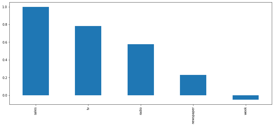
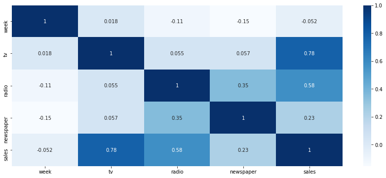
To examine the data we’re dealing with, and to check whether they are any identifiable correlations between marketing activity and sales, we can use describe() and corr(). This company is spending large amounts on TV and radio advertising, which are both highly correlated with sales revenue. Newspapers, by contrast, deliver far less.
What we are looking for is a linear relationship between the marketing budgets assigned to each channel, and the sales revenue that comes out the other end. You would hope that spending more on certain types of marketing would lead to greater sales, but perhaps some channels support others, and that people who hear a radio ad for a business they read about in the newspaper may be more likely to purchase.
df.describe().T
| count | mean | std | min | 25% | 50% | 75% | max | |
|---|---|---|---|---|---|---|---|---|
| week | 200.0 | 99.5000 | 57.879185 | 0.0 | 49.750 | 99.50 | 149.250 | 199.0 |
| tv | 200.0 | 147.0425 | 85.854236 | 0.7 | 74.375 | 149.75 | 218.825 | 296.4 |
| radio | 200.0 | 23.2640 | 14.846809 | 0.0 | 9.975 | 22.90 | 36.525 | 49.6 |
| newspaper | 200.0 | 30.5540 | 21.778621 | 0.3 | 12.750 | 25.75 | 45.100 | 114.0 |
| sales | 200.0 | 14.0225 | 5.217457 | 1.6 | 10.375 | 12.90 | 17.400 | 27.0 |
plt.figure(figsize=(15,6))
bars = df.corr()['sales'].sort_values(ascending=False).plot(kind='bar')
plt.figure(figsize=(15,6))
heatmap = sns.heatmap(df.corr(), annot=True, cmap="Blues")
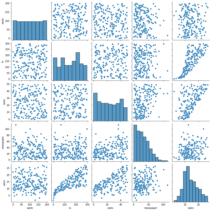
Seaborn’s pairplot() function is a great way to quickly visualise the data. As you can see from the scatter plots,
there are some clear correlations between marketing spend for the channels and sales for the business, so we should
be able to make some good predictions when we get to that stage. Our marketing variables are definitely correlated
with sales revenue - some more than others.
sns.pairplot(df)
<seaborn.axisgrid.PairGrid at 0x7f4748449dd0>
Create training and test data
Next, we’ll create our training and test datasets from the original dataframe. For the X dataset, we’re including all the features apart from sales, while in the y dataset we’re including only the target sales variable. As usual, we’ll use the scikit-learn train_test_split() function to randomly assign data, and have allocated 30% of the data to the test group.
X = df[['week', 'tv', 'radio', 'newspaper']]
y = df['sales']

X_train, X_test, y_train, y_test = train_test_split(X, y, test_size=0.3, random_state=0)
Scale the data
To help improve the model results, it’s worth using a scaling or normalisation technique on the data, especially if it’s skewed. Ours is not too bad, but I’ve passed it through StandardScaler() to be sure.
scaler = StandardScaler()
X_train = scaler.fit_transform(X_train)
X_test = scaler.transform(X_test)
Identify the best model
Next, we’ll test a load of different regression models to see which one delivers the best results. Spoiler alert: It’s nearly always XGBRegressor! The quickest and easiest way to do this is to place all the model parameters in a Python dictionary and then loop over them. Here’s the dictionary of models to test.
regressors = {
    "XGBRegressor": XGBRegressor(),
    "RandomForestRegressor": RandomForestRegressor(),
    "DecisionTreeRegressor": DecisionTreeRegressor(),
    "GaussianProcessRegressor": GaussianProcessRegressor(),
    "SVR": SVR(),
    "NuSVR": NuSVR(),
    "LinearSVR": LinearSVR(),
    "KernelRidge": KernelRidge(),
    "LinearRegression": LinearRegression(),
    "Ridge":Ridge(),
    "Lars": Lars(),
    "TheilSenRegressor": TheilSenRegressor(),
    "HuberRegressor": HuberRegressor(),
    "PassiveAggressiveRegressor": PassiveAggressiveRegressor(),
    "ARDRegression": ARDRegression(),
    "BayesianRidge": BayesianRidge(),
    "ElasticNet": ElasticNet(),
    "OrthogonalMatchingPursuit": OrthogonalMatchingPursuit(),
}
We’ll create a Pandas dataframe called df_models and now loop through the regressors, fit each one to the data, and return the Root Mean Squared Error of a 10-fold cross validation to the dataframe, and then display the output.
df_models = pd.DataFrame(columns=['model', 'run_time', 'rmse', 'rmse_cv'])

for key in regressors:

    print('*',key)

    start_time = time.time()

    regressor = regressors[key]
    model = regressor.fit(X_train, y_train)
    y_pred = model.predict(X_test)

    scores = cross_val_score(model,
                             X_train,
                             y_train,
                             scoring="neg_mean_squared_error",
                             cv=10)

    row = {'model': key,
           'run_time': format(round((time.time() - start_time)/60,2)),
           'rmse': round(np.sqrt(mean_squared_error(y_test, y_pred))),
           'rmse_cv': round(np.mean(np.sqrt(-scores)))
    }

    df_models = df_models.append(row, ignore_index=True)
* XGBRegressor
* RandomForestRegressor
* DecisionTreeRegressor
* GaussianProcessRegressor
* SVR
* NuSVR
* LinearSVR
* KernelRidge
* LinearRegression
* Ridge
* Lars
* TheilSenRegressor
* HuberRegressor
* PassiveAggressiveRegressor
* ARDRegression
* BayesianRidge
* ElasticNet
* OrthogonalMatchingPursuit
Perhaps unsurprisingly, XGBRegressor came out on top, but the RandomForest model also worked very well.
df_models.head(20).sort_values(by='rmse_cv', ascending=True)
| model | run_time | rmse | rmse_cv | |
|---|---|---|---|---|
| 0 | XGBRegressor | 0.01 | 1 | 1 |
| 1 | RandomForestRegressor | 0.02 | 1 | 1 |
| 2 | DecisionTreeRegressor | 0.0 | 2 | 1 |
| 15 | BayesianRidge | 0.0 | 2 | 2 |
| 14 | ARDRegression | 0.0 | 2 | 2 |
| 13 | PassiveAggressiveRegressor | 0.0 | 3 | 2 |
| 12 | HuberRegressor | 0.0 | 2 | 2 |
| 11 | TheilSenRegressor | 0.04 | 2 | 2 |
| 10 | Lars | 0.0 | 2 | 2 |
| 8 | LinearRegression | 0.0 | 2 | 2 |
| 6 | LinearSVR | 0.0 | 2 | 2 |
| 5 | NuSVR | 0.0 | 2 | 2 |
| 4 | SVR | 0.0 | 2 | 2 |
| 3 | GaussianProcessRegressor | 0.0 | 2 | 2 |
| 9 | Ridge | 0.0 | 2 | 2 |
| 16 | ElasticNet | 0.0 | 3 | 3 |
| 17 | OrthogonalMatchingPursuit | 0.0 | 3 | 3 |
| 7 | KernelRidge | 0.0 | 14 | 15 |
Assess the best model
To assess the best model we can re-fit the data and generate a new set of predictions. To get further improvements, you could also try tuning the model parameters to see if the score improves.
regressor = XGBRegressor()
model = regressor.fit(X_train, y_train)
y_pred = model.predict(X_test)
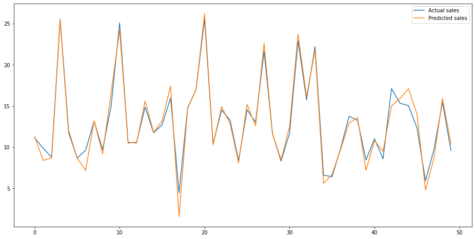
Finally, we’ll merge the predictions to our original data and plot the predicted sales versus the actual sales. As you can see, the model is pretty good at estimating the sales revenue a given mix of spend on marketing channels will generate.
test = pd.DataFrame({'Predicted sales':y_pred, 'Actual sales':y_test})
fig= plt.figure(figsize=(16,8))
test = test.reset_index()
test = test.drop(['index'],axis=1)
plt.plot(test[:50])
plt.legend(['Actual sales','Predicted sales'])
Next steps
This model works, fairly well, but it’s only crude given the complexity of many MMMs. To further improve this, there
are a whole load of other things we could do. Firstly, we could add some lagged data, by using shift to get the
channel spend in the previous weeks to see if that’s correlated to sales in future periods. We could also do some
hyperparameter tuning, or add in some additional regressors if we have them.
Since marketing results are based on the four Ps - Price, Product, Place, Promotion - if you have access to them, your regressors really ought to include data on these important variables.
To use the model, we can apply a simple “what if” technique to adjust the spend on the marketing channels and see what happens to the sales predicted. While not a perfect solution, it’s usually sufficient to give you a decent idea of what’s likely to happen if you reduce or increase the marketing spend on a channel.
Matt Clarke, Monday, May 03, 2021


Other posts you might like

How to tune a LightGBMClassifier model with Optuna
The LightGBM model is a gradient boosting framework that uses tree-based learning algorithms, much like the popular XGBoost model. LightGBM supports both classification and regression tasks, and is known for...

How to create a customer retention model with XGBoost
Although all business know the importance of retaining customers, few companies are actually able to measure customer retention accurately, and fewer still can predict which ones will churn or be...
