How to create a decision tree classification model using scikit-learn
Learn how to create a decision tree classification model using scikit-learn in Python with the sklearn DecisionTreeClassifier in this basic tutorial with example code.

The Decision Tree or DT is one of the most well known and most widely used supervised machine learning algorithms and can be applied to both regression and classification. As the name suggests, a decision tree model aims to predict the value of a target variable using decision rules it infers from the training data.
Since the decision tree is a tree-based model, you can also export the decision tree itself to help you explain the model’s output. Model explainability or model interpretability is often a useful feature to have, especially in business, where some stakeholders might be untrusting of a black box algorithm where nobody really understands what it’s doing or how it works.
In this simple Python example, we’ll build a basic decision tree classification model using scikit-learn. We’ll be using the built-in DecisionTreeClassifier to create a decision tree model for multi-class classification. We’ll fit it to our data, evaluate the model performance, and then do some basic model hyperparameter tuning. Let’s get started.
Load the packages
To get started open a Jupyter notebook and import the packages below from scikit-learn. We’ll be using the sklearn DecisionTreeClassifier to create our decision tree classification model, the train_test_split function to split the data into our training and test datasets, and the accuracy_score and classification_report functions to evaluate our model’s performance. To save the hassle of data cleansing and feature engineering we’ll use one of scikit-learn’s test datasets on the chemistry of different wines.
from sklearn.tree import DecisionTreeClassifier
from sklearn.model_selection import KFold
from sklearn.model_selection import cross_val_score
from sklearn.model_selection import train_test_split
from sklearn.metrics import accuracy_score
from sklearn.metrics import classification_report
from sklearn.datasets import load_wine
from sklearn import tree
import matplotlib.pyplot as plt
Load the data
Next, we’ll use the load_wine() function to load the wine dataset and return the X training data and the y target variable. Passing as_frame=True will return the data as a Pandas dataframe so we can inspect it more easily. Load up a sample() of five rows to see what we’re working with. The y data is a series containing an index and an integer value denoting the class of each sample in the dataset.
If you’re using your own data, you’ll need to first prepare your data for use in the model by preprocessing it. As you can see from the below data, all values in the training data need to be converted to a numeric format - either a float or an integer.
You will need to encode categorical variables them to make them numeric. You might also want to apply some feature engineering techniques to guide the model by creating potentially useful values that can be used to help predict the target variable.
X, y = load_wine(return_X_y=True, as_frame=True)
X.sample(5)
| alcohol | malic_acid | ash | alcalinity_of_ash | magnesium | total_phenols | flavanoids | nonflavanoid_phenols | proanthocyanins | color_intensity | hue | od280/od315_of_diluted_wines | proline | |
|---|---|---|---|---|---|---|---|---|---|---|---|---|---|
| 17 | 13.83 | 1.57 | 2.62 | 20.0 | 115.0 | 2.95 | 3.40 | 0.40 | 1.72 | 6.60 | 1.13 | 2.57 | 1130.0 |
| 155 | 13.17 | 5.19 | 2.32 | 22.0 | 93.0 | 1.74 | 0.63 | 0.61 | 1.55 | 7.90 | 0.60 | 1.48 | 725.0 |
| 131 | 12.88 | 2.99 | 2.40 | 20.0 | 104.0 | 1.30 | 1.22 | 0.24 | 0.83 | 5.40 | 0.74 | 1.42 | 530.0 |
| 73 | 12.99 | 1.67 | 2.60 | 30.0 | 139.0 | 3.30 | 2.89 | 0.21 | 1.96 | 3.35 | 1.31 | 3.50 | 985.0 |
| 128 | 12.37 | 1.63 | 2.30 | 24.5 | 88.0 | 2.22 | 2.45 | 0.40 | 1.90 | 2.12 | 0.89 | 2.78 | 342.0 |
y.sample(5)
119    1
134    2
78     1
168    2
52     0
Name: target, dtype: int64
Split into training and test datasets
Now we have our X and y data we can pass it to the scikit-learn train_test_split() function to create the training and test data we need to train and evaluate our classification model. We’ll set the test_size value to 0.3 so that 30% of our data is used for testing and the rest for training. Setting the random_state value ensures results are more reproducible between runs.
X_train, X_test, y_train, y_test = train_test_split(X, y, test_size=0.3, random_state=1)
Create and fit the model
Next, we’ll create our decision tree model using DecisionTreeClassifier. To ensure reproducible results between runs, we’ll pass a value to the random_state argument. If you don’t do this, you’ll get a slightly different result each time you run the model. To keep things simple, we’re first going to fit a base model with no additional optional arguments passed, apart from the random_state value.
model = DecisionTreeClassifier(random_state=1)
Now we’ll “fit” the data to our model by passing in the X_train data, which includes only the features for the training portion of 70% of the overall dataset, and the separate y_train target variables for the same dataset. The decision tree algorithm will use the training data to work out what decision rules are required to get the best results at predicting the target variable.
model.fit(X_train, y_train)
DecisionTreeClassifier(random_state=1)
Generate predictions
Now we’ve built our model by fitting it on the training data, we can pass it the X_test data. It’s never seen this data before, as it’s only been trained using the 70% portion of training data, so we’ll now see how well the model “generalises” and is capable of predicting the target variable on unseen data. Here’s the X_test data we’re passing to the model.
X_test.head()
| alcohol | malic_acid | ash | alcalinity_of_ash | magnesium | total_phenols | flavanoids | nonflavanoid_phenols | proanthocyanins | color_intensity | hue | od280/od315_of_diluted_wines | proline | |
|---|---|---|---|---|---|---|---|---|---|---|---|---|---|
| 161 | 13.69 | 3.26 | 2.54 | 20.0 | 107.0 | 1.83 | 0.56 | 0.50 | 0.80 | 5.88 | 0.96 | 1.82 | 680.0 |
| 117 | 12.42 | 1.61 | 2.19 | 22.5 | 108.0 | 2.00 | 2.09 | 0.34 | 1.61 | 2.06 | 1.06 | 2.96 | 345.0 |
| 19 | 13.64 | 3.10 | 2.56 | 15.2 | 116.0 | 2.70 | 3.03 | 0.17 | 1.66 | 5.10 | 0.96 | 3.36 | 845.0 |
| 69 | 12.21 | 1.19 | 1.75 | 16.8 | 151.0 | 1.85 | 1.28 | 0.14 | 2.50 | 2.85 | 1.28 | 3.07 | 718.0 |
| 53 | 13.77 | 1.90 | 2.68 | 17.1 | 115.0 | 3.00 | 2.79 | 0.39 | 1.68 | 6.30 | 1.13 | 2.93 | 1375.0 |
To generate predictions from the model, we’ll append the predict() function to our DecisionTreeClassifier, which we stored in a variable called model, along with the X_test dataframe. We’ll assign the output to a variable called y_pred, to denote that these are the prediction y target variables. If you print y_pred you’ll see that a numpy array is returned that contains 0, 1, or 2, which maps to the class for each predicted value.
y_pred = model.predict(X_test)
y_pred
array([2, 1, 0, 1, 0, 2, 1, 0, 2, 1, 0, 1, 1, 0, 1, 1, 2, 0, 1, 0, 0, 1,
       2, 0, 0, 2, 0, 0, 0, 2, 1, 2, 2, 0, 1, 1, 1, 1, 1, 0, 0, 2, 2, 0,
       0, 0, 1, 0, 0, 0, 1, 2, 2, 0])
Evaluate model performance
Now we’ve generated our predictions, we need to evaluate the model’s performance to see if it was any good. There are many different evaluation metrics that you can use to assess the performance of a machine learning model. We’ll first use the accuracy_score() metric. To use this you need to pass it the actual values stored in y_test and the predicted values stored in y_pred. The accuracy_score() metric will then return a percentage score showing the proportion of results that we predicted correctly. Our base model decision tree classifier scores 94.4%.
accuracy = accuracy_score(y_test, y_pred)
accuracy
0.9444444444444444
Another useful metric for evaluating a classification model is the classification report, which can be accessed via the classification_report() function. This works in the same way as the other scikit-learn model evaluation metric functions, so you just need to pass it the same y_test and y_pred data. To make it print the results neatly, you’ll need to wrap the output in a print() statement, even inside a Jupyter notebook.
print(classification_report(y_test, y_pred))
              precision    recall  f1-score   support

           0       0.96      0.96      0.96        23
           1       0.94      0.89      0.92        19
           2       0.92      1.00      0.96        12

    accuracy                           0.94        54
   macro avg       0.94      0.95      0.95        54
weighted avg       0.94      0.94      0.94        54
The classification report can seem a bit confusing the first time you use it. The first column, which contains the 0, 1, and 2 values, shows the target variables predicted along with their evaluation metric scores. It’s fairly normal for a model to be good at predicting some target variables but less good at predicting others, and that’s what we’re seeing here. Four metrics are returned - precision, recall, F1 score, and support. Here’s what they mean.
| Metric | Definition |
|---|---|
| Precision | The precision model evaluation metric is the ratio of true positives over true positives plus false positives, i.e. precision = tp / (tp + fp). Precision shows the model's ability not to label a negative sample as positive. |
| Recall | The recall model evaluation metric is the ratio of true positives over true positives plus false negatives, i.e. precision = tp / (tp + fp). Recall shows the model's ability to detect the positive samples. |
| F1 score | The F1 score (or F-beta score, as it's also known) is a weighted harmonic mean of the precision and recal scores, where an F-beta score of 1 is best and 0 is worst. |
| Support | The support value shows the number of occurrences of each class in the `y_true` (or `y_test`) data. |
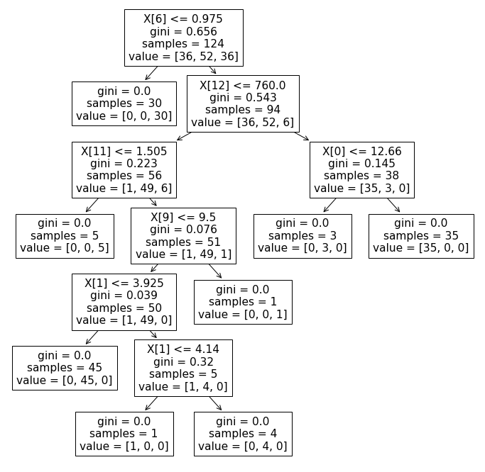
Plot the decision tree
One neat feature of the decision tree model is that the results are interpretable, since it’s just a tree-based model of decision rules. To generate the tree used within the decision tree model, you can pass the model object to tree.plot_model(). To increase the size of the image plot_tree() generates, I’d recommend using Matplotlib to force the size of the figure to something more readable using plt.figure(figsize=(12,12)).
plt.figure(figsize=(12,12))
tree.plot_tree(model)
[Text(251.10000000000002, 605.7257142857143, 'X[6] <= 0.975\ngini = 0.656\nsamples = 124\nvalue = [36, 52, 36]'),
 Text(167.4, 512.537142857143, 'gini = 0.0\nsamples = 30\nvalue = [0, 0, 30]'),
 Text(334.8, 512.537142857143, 'X[12] <= 760.0\ngini = 0.543\nsamples = 94\nvalue = [36, 52, 6]'),
 Text(167.4, 419.34857142857146, 'X[11] <= 1.505\ngini = 0.223\nsamples = 56\nvalue = [1, 49, 6]'),
 Text(83.7, 326.16, 'gini = 0.0\nsamples = 5\nvalue = [0, 0, 5]'),
 Text(251.10000000000002, 326.16, 'X[9] <= 9.5\ngini = 0.076\nsamples = 51\nvalue = [1, 49, 1]'),
 Text(167.4, 232.9714285714286, 'X[1] <= 3.925\ngini = 0.039\nsamples = 50\nvalue = [1, 49, 0]'),
 Text(83.7, 139.7828571428571, 'gini = 0.0\nsamples = 45\nvalue = [0, 45, 0]'),
 Text(251.10000000000002, 139.7828571428571, 'X[1] <= 4.14\ngini = 0.32\nsamples = 5\nvalue = [1, 4, 0]'),
 Text(167.4, 46.594285714285775, 'gini = 0.0\nsamples = 1\nvalue = [1, 0, 0]'),
 Text(334.8, 46.594285714285775, 'gini = 0.0\nsamples = 4\nvalue = [0, 4, 0]'),
 Text(334.8, 232.9714285714286, 'gini = 0.0\nsamples = 1\nvalue = [0, 0, 1]'),
 Text(502.20000000000005, 419.34857142857146, 'X[0] <= 12.66\ngini = 0.145\nsamples = 38\nvalue = [35, 3, 0]'),
 Text(418.5, 326.16, 'gini = 0.0\nsamples = 3\nvalue = [0, 3, 0]'),
 Text(585.9, 326.16, 'gini = 0.0\nsamples = 35\nvalue = [35, 0, 0]')]
Next steps
In this very simple example we’ve used Python’s scikit-learn package to create a decision tree classifier. While this approach works, it’s a simplification of what you’d do when creating a more robust model. In a real world scenario you’ll get better results from testing a range of different classification algorithms and then using an approach called model selection with cross validation.
This approach to model selection will help you identify the model best suited to your problem and which provides the highest level of accuracy (or whatever metric you choose to evaluate using). Applying model selection can often give you significant boosts in performance.
Once you’ve selected your classification algorithm, the final step is to tune your model using a technique called hyperparameter tuning. This tweaks the model’s specific settings to fine tune the performance. While it rarely leads to big improvements, it can give you a little extra boost and is usually worthwhile, especially if you set it up and leave it to run overnight.
Matt Clarke, Sunday, May 01, 2022


Other posts you might like

How to tune a LightGBMClassifier model with Optuna
The LightGBM model is a gradient boosting framework that uses tree-based learning algorithms, much like the popular XGBoost model. LightGBM supports both classification and regression tasks, and is known for...

How to create a customer retention model with XGBoost
Although all business know the importance of retaining customers, few companies are actually able to measure customer retention accurately, and fewer still can predict which ones will churn or be...
