How to create synthetic data sets for machine learning

Dummies by Sarah Kurfeß, Unsplash.

16 minutes to read

While there are many open source datasets available for you to use when learning new data science techniques, sometimes you may struggle to find a data set to use to learn your chosen technique or train your specific model.

Thankfully, it’s actually fairly simple to create artificial, synthetic or dummy datasets using only Pandas and Numpy. With some creativity, you can generate synthetic data sets that resemble real world data and you can even control the statistical distributions if you wish.

There are loads of different ways to create dummy data. Let’s take a look at some of the most simple technique you can use to create an artificial ecommerce data set using only Pandas and Numpy.

1. Creating a data frame of unique customers

Our first step is to create a Pandas data frame containing unique customer IDs for each of our fake customers. We’ll use np.random.randint() to create a unique integer value between 1 and 100,000 and then assign it to each of our customers in a column called customer_id.

import pandas as pd
import numpy as np

items = 100000
customer_id = np.random.randint(1, 100000, items)

df = pd.DataFrame({"customer_id":customer_id})
df.head()

	customer_id
0	9174
1	98068
2	62786
3	36540
4	25742

2. Creating dummy categorical variables

Next we’ll use the random.choice() function in Numpy to create a gender column containing 49% in male and female and 2% in other, and a type column in which 36% of customers are new and 64% are returning, then we’ll add these to our dataframe.

df['gender'] = np.random.choice(["male","female", "other"], size=items, p=[.49,.49,.02])
df['type'] = np.random.choice(["new","returning"], size=items, p=[.36,.64])

df.head()

	customer_id	gender	type
0	9174	female	returning
1	98068	male	returning
2	62786	male	new
3	36540	male	new
4	25742	male	returning

3. Create dummy binary variables

Now we’ll add some binary variables to simulate one-hot encoded or label encoded data. We’ll add a complained column in which 5% of customers have a 1 and 95% have a zero, and we’ll randomly assign a value between 1 and 5 to each customer in the segment column.

df['complained'] = np.random.choice([1, 0], size=items, p=[.05,.95])
df['segment'] = np.random.choice([1, 2, 3, 4, 5], size=items, p=[.2,.2,.2,.2,.2])

df.sample(10)

	customer_id	gender	type	segment
91772	55712	female	new	4
20345	57934	other	returning	3
18579	35286	male	returning	3
1162	57650	female	returning	3
83295	51486	female	returning	5
92511	71999	female	returning	3
90956	12445	other	new	2
45773	51319	male	new	5
1901	73737	male	returning	2
5610	36660	male	new	4

3. Create dummy numeric data

For our customer metric data, such as our synthetic recency, frequency, and monetary data, we will use np.random.randint() and np.random.uniform() to create data that looks like real customer data.

df['recency'] = np.random.randint(1, 1000, items)
df['frequency'] = np.random.randint(1, 50, items)
df['monetary'] = np.random.uniform(19.99, 9999.99, items)

df.sample(10)

	customer_id	gender	type	complained	segment	recency	frequency	monetary
41618	68380	male	returning	0	2	770	23	1388.614746
93970	23898	female	returning	0	5	41	42	4543.883058
72267	96191	male	returning	0	3	67	17	5912.788236
88265	51647	male	returning	0	5	485	31	6844.415058
36901	1885	female	new	1	3	622	36	5374.382082
71719	32143	other	returning	0	3	14	36	8762.230686
58465	29517	female	returning	0	4	758	23	1326.652237
37604	82762	female	new	0	5	113	49	1133.411517
45707	20113	female	new	0	1	795	35	5207.388227
12591	81603	male	returning	0	4	530	38	678.581544

Creating data for classification models

The other way to quickly create datasets is to use the tools within Scikit-Learn. This gives you less control over the data created, but it’s much quicker and you can easily control which features are informative (and important to the model) or redundant (and unimportant to the model).

For classification models, you can create artificial datasets in Scikit-Learn using the make_classification() function. Here we’ll set it to create 1000 samples with 100 features, 10 of these will be informative, and 3 will be redundant. We’ll define two classes and we’ll assign 10% of the results to one class and 90% to the other.

import pandas as pd
from sklearn.datasets import make_classification

features, output = make_classification(n_samples = 1000,
                                       n_features = 100,
                                       n_informative = 10,
                                       n_redundant = 3,
                                       n_classes = 2,
                                       weights = [.1, .9],
                                       random_state=0
                                      )

pd.DataFrame(features).head()

	0	1	2	3	4	5	6
0	-1.890027	1.372168	0.938193	-0.619863	0.131079	1.171468	1.819417
1	0.575108	0.253721	-1.578379	-0.993457	1.746113	1.706953	0.004448
2	0.588039	-0.103351	1.651014	-0.682294	-2.010642	0.991115	-0.516709
3	-1.795687	0.297395	-0.931469	-0.938651	0.369023	-0.072191	-2.292341
4	0.985046	0.527223	-0.445843	-0.421475	-1.168308	1.857537	1.857537

5 rows × 100 columns

pd.DataFrame(output).sample(10)

	0
988	1
384	1
944	1
556	1
228	1
310	1
465	0
638	0
248	1
85	1

Creating data for regression models

You can create artificial datasets for regression models in a similar way using the make_regression() function. In this example we’re creating 1000 samples with five features, three of which are informative to the model. We’ve got one regression target and haven’t added any Gaussian noise to the data. Passing the coef = True argument gives us the raw output coefficients from the model.

import pandas as pd
from sklearn.datasets import make_regression

features, output, coef = make_regression(n_samples = 1000,
                                   n_features = 5,
                                   n_informative = 3,
                                   n_targets = 1,
                                   noise = 0,
                                   coef = True
                                   )

pd.DataFrame(features, columns=['Organic', 'Paid', 'Social', 'Direct', 'Email']).head()

	Organic	Paid	Social	Direct	Email
0	0.126290	0.080609	-0.678113	1.080924	-1.028701
1	0.185861	0.724501	1.251502	-0.045964	-0.495496
2	0.512126	0.818959	0.727368	1.464926	-0.227964
3	-0.896851	-0.451308	0.152532	-0.903700	-0.313880
4	0.083517	-0.847535	1.349897	-1.608228	-0.276973

pd.DataFrame(output, columns=['Profit']).head()

	Profit
0	-18.804014
1	28.436600
2	54.506685
3	-44.576138
4	-73.214960

pd.DataFrame(coef, columns=['Coefficients'])

	Coefficients
0	0.000000
1	61.191764
2	0.000000
3	7.877698
4	31.351953

Create data for clustering models

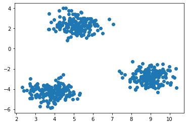
Finally, for clustering models, such as K-means, we can construct synthetic clustering datasets by using make_blobs(). Here we’ll create a dataset comprising 500 samples with three features and three clusters. We’ll shuffle the data and add a standard deviation of 0.6 to the clusters.

import matplotlib.pyplot as plt
from sklearn.datasets import make_blobs

X, y = make_blobs(n_samples = 500,
                  n_features = 3,
                  centers = 3,
                  cluster_std = 0.6,
                  shuffle = True
                 )

Since we can’t easily view these clusters in a dataframe, we’ll use matplotlib to create a scatter plot showing their positions in space. This gives us three clear clusters for our model to identify.

plt.scatter(X[:,0], X[:,1])
plt.show()

png

Create a dataframe with a time series index

The Pandas util module is another great way to quickly generate dummy data for your projects. It allows you to create various forms of data to your specifications. To construct a dataframe of time series data you can use pd.util.testing.makeTimeDataFrame().

df = pd.util.testing.makeTimeDataFrame()
df.head()

	A	B	C	D
2000-01-03	-0.316010	0.016499	0.388287	0.817572
2000-01-04	0.226709	0.275672	1.127386	-0.326969
2000-01-05	-0.136579	0.869829	-1.136967	-1.227729
2000-01-06	-0.790527	-0.765968	0.744052	-0.942392
2000-01-07	0.016989	-0.646809	1.799815	0.487903

Create a test dataframe containing missing values

In many cases I’ve needed a Pandas dataframe that contains missing values, so have gone to the hassle of finding a dataset I like and then randomly removing values. However, the Pandas makeMissingDataframe() function actually does this for you!

df = pd.util.testing.makeMissingDataframe()
df.head()

	A	B	C	D
835sD6b9XV	0.298557	0.635936	0.158512	-2.576662
UPbjKlZIl5	NaN	-1.800019	-0.712900	-0.145401
w1DpovhuLP	-0.109157	-1.139069	1.682762	0.074845
GeWPq2Avlt	0.818799	0.033064	-1.319938	-0.893519
gVZxWkU5IN	-0.725306	NaN	0.344579	NaN

Create a test dataframe containing mixed values

You can also create dataframes containing mixed values using the regular makeDataFrame() function which is also in pd.util.testing.

df = pd.util.testing.makeDataFrame()
df.head()

	A	B	C	D
ewdRytN6pe	1.038578	-0.617057	0.922791	-1.651699
KEKPyZLxcW	0.242627	-1.942784	-0.708247	0.579638
jwTOMzI2I0	-0.326679	1.874722	1.678302	0.118675
7JPnSlV7kV	-0.870648	2.079954	0.590904	0.948251
5yMGxJfWcj	0.594368	-2.288743	-1.787830	-0.750000

Matt Clarke, Thursday, March 04, 2021

Matt Clarke Matt is an Ecommerce and Marketing Director who uses data science to help in his work. Matt has a Master's degree in Internet Retailing (plus two other Master's degrees in different fields) and specialises in the technical side of ecommerce and marketing.