How to make time series forecasts with Neural Prophet
The Neural Prophet time series forecasting model was developed by Facebook and is a powerful tool for predicting future events. Here's how you can use it to forecast your web traffic using Google Analytics.

The Neural Prophet model is relatively new and was heavily inspired by Facebook’s earlier Prophet time series forecasting model. NeuralProphet is a neural network based model that uses a PyTorch backend, and has been designed with a modular architecture, allowing extra features to be bolted on in the future.
In this project I’ll show you the basics to get you started with forecasting using NeuralProphet. We’ll fetch some historical Google Analytics traffic data for my site, and use it to predict what will happen to the traffic over the coming year. Let’s get started!
Install the packages
For this project we’ll be using the NeuralProphet time series forecasting model developed by Facebook, and the GAPandas Google Analytics API module I created. To install these, open a Jupyter notebook and enter the commands below in a code cell and execute it by pressing shift and enter. NeuralProphet uses Torch, which is quite a hefty package, so expect the install to take a few minutes.
!pip3 install neuralprophet[live]
!pip3 install gapandas
Load the packages
Next, import the Pandas and GAPandas packages so we can extract data from Google Analytics and manipulate it using Pandas. Then, from neuralprophet, import the NeuralProphet module and set_random_seed. Initialise set_random_seed() with a random value to ensure your results are reproducible on subsequent model runs.
import pandas as pd
import gapandas as gp
from neuralprophet import NeuralProphet
from neuralprophet import set_random_seed
set_random_seed(0)
Configure GAPandas
To fetch data from your Google Analytics account you will need to have a client secrets JSON key file to authenticate yourself. You can obtain one of these from the Google Search Console. You’ll also need the view ID for the GA property you want to query, and the start and end date for your window. I’d suggest selecting as much data as you have, in order to give the model the best chance of success.
key_ga = "client_secrets.json"
view_ga = "1234567890"
start_date = "2016-01-01"
end_date = "2021-05-01"
Fetch your Google Analytics data
Pass the file path of your client secrets JSON keyfile to the get_service() function and assign the service object to a variable, then create a payload dictionary to pass to the API. Here we’re just fetching the number of sessions for each date in our window.
Finally, use run_query() to pass the service object, the view ID, and the payload dictionary back to Google Analytics. This will return your API query results in a Pandas dataframe.
service = gp.get_service(key_ga)

payload = {
    'start_date': start_date,
    'end_date': end_date,
    'metrics': 'ga:sessions',
    'dimensions': 'ga:date'
}

df = gp.run_query(service, view_ga, payload)
df.head()
| date | sessions | |
|---|---|---|
| 0 | 2016-01-01 | 7 |
| 1 | 2016-01-02 | 2 |
| 2 | 2016-01-03 | 2 |
| 3 | 2016-01-04 | 1 |
| 4 | 2016-01-05 | 6 |
Reformat data for Neural Prophet model
Like its predecessor FBProphet, Neural Prophet also requires that you do some simple reformatting of your Pandas
dataframe before it is passed to the model. All you need to do is ensure that the column containing the date is of
the correct type and that the columns are labelled ds (for the date stamp) and y for the target parameter you wish to predict.
data = df.rename(columns={'date': 'ds', 'sessions': 'y'})[['ds', 'y']]
data.head()
| ds | y | |
|---|---|---|
| 0 | 2016-01-01 | 7 |
| 1 | 2016-01-02 | 2 |
| 2 | 2016-01-03 | 2 |
| 3 | 2016-01-04 | 1 |
| 4 | 2016-01-05 | 6 |
Create a simple model
There are loads of different options you can pass to Neural Prophet to help improve results. For now, we’ll keep things simple and just build a baseline model. To do this we initialise NeuralProphet() and then fit it to our data using the daily D frequency.
model = NeuralProphet(daily_seasonality=False)
metrics = model.fit(data, freq="D")
INFO: nprophet.config - set_auto_batch_epoch: Auto-set batch_size to 32
INFO: nprophet.config - set_auto_batch_epoch: Auto-set epochs to 32


  0%|          | 0/100 [00:00<?, ?it/s]


INFO: nprophet - _lr_range_test: learning rate range test found optimal lr: 2.85E-01
Epoch[32/32]: 100%|██████████| 32/32 [00:02<00:00, 15.30it/s, SmoothL1Loss=0.00585, MAE=72.3, RegLoss=0]
Generate predictions from the model
To generate predictions from the model, we first need to create a future dataframe. As the name suggests, this is a new dataframe of dates that extend your original dataframe’s dates X periods into the future. Since ours is set to daily, this will extend our dataframe by 90 days. Once the future dataframe is created, we can pass that to the predict() function to return a forecast.
future = model.make_future_dataframe(data, periods=90)
forecast = model.predict(future)
The predict() function returns a Pandas dataframe containing the dates in the future and identifies the yhat1 prediction, as well as the trend, season_yearly, and season_weekly. It’s common for the y and residual1 values to contain NaN values.
forecast.head()
| ds | y | yhat1 | residual1 | trend | season_yearly | season_weekly | |
|---|---|---|---|---|---|---|---|
| 0 | 2021-05-02 | None | 864.840271 | NaN | 799.754761 | 28.044598 | 37.040867 |
| 1 | 2021-05-03 | None | 857.137024 | NaN | 800.181152 | 31.580545 | 25.375282 |
| 2 | 2021-05-04 | None | 844.785583 | NaN | 800.607483 | 35.279961 | 8.898128 |
| 3 | 2021-05-05 | None | 828.126343 | NaN | 801.033936 | 39.125648 | -12.033257 |
| 4 | 2021-05-06 | None | 828.524902 | NaN | 801.460266 | 43.099255 | -16.034576 |
Show the time series components
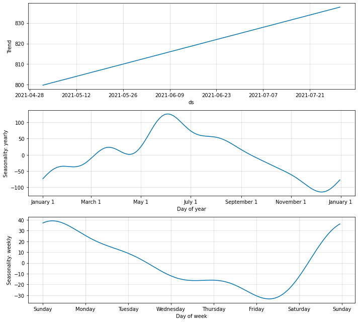
Since a time series forecast is impacted by the trend, the yearly seasonality, and the daily seasonality, it’s useful to extract these to see what lies beneath. This process is known as time series decomposition, and NeuralProphet makes it very simple. Just pass the forecast dataframe to plot_components() and it will show you the decomposed data. This reveals a nice upward trend for my site, and shows that it’s busiest in June, with Sundays being the busiest weekday.
components = model.plot_components(forecast)
Plot the forecast
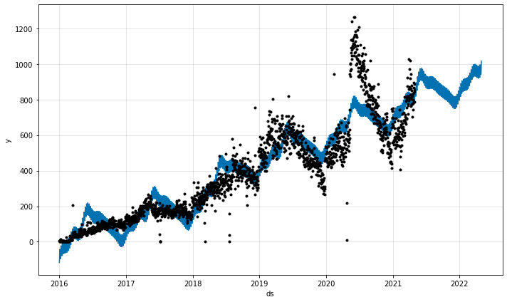
Next, let’s re-run the model with a longer future dataframe. This time, we’ll extend it to 365 days to observe what the model thinks my site’s traffic will do over the next year. When it runs, the model will make predictions for past periods to help it learn what will happen in the future. The blue line represents the 95% confidence interval for the model’s predictions, and the black dots represent the actual data.
Since my site is about fly fishing, it’s strongly tied to the weather (and pandemic-related lockdowns that prevent or re-allow fishing), so some of the later predictions fall quite a way off the actual results. This is probably unavoidable, but adding an additional weather regressor may help put the model back on track.
future = model.make_future_dataframe(data, periods=365, n_historic_predictions=True)
forecast = model.predict(future)
model.plot(forecast)
There’s much more than you can do with NeuralProphet than this, but hopefully this is plenty to get you started, so you can adjust the model parameters and add regressors that help improve the forecast predictions.
In my experience NeuralProphet works very well - slightly better than the original FBProphet model. However, it currently lacks some useful features present in regular FBProphet, so I’d recommend you try both until the stable version of NeuralProphet is out.
Matt Clarke, Sunday, May 02, 2021


Other posts you might like

How to tune a LightGBMClassifier model with Optuna
The LightGBM model is a gradient boosting framework that uses tree-based learning algorithms, much like the popular XGBoost model. LightGBM supports both classification and regression tasks, and is known for...

How to create a customer retention model with XGBoost
Although all business know the importance of retaining customers, few companies are actually able to measure customer retention accurately, and fewer still can predict which ones will churn or be...
