How to forecast Google Trends search data with NeuralProphet
Google Trends data can give retailers insight into the growth or decline of searches in the wider market. Here's how to forecast them using NeuralProphet and PyTrends.

In ecommerce, it is often difficult to tell whether your search traffic is performing to expectations. What your boss perceives to be caused by an on-site or marketing-related issue may well be caused by a downturn in search traffic for the phrase in question.
Thankfully, Google Trends data makes it possible to understand the general search market outside your website, and can help you understand whether trends you’ve observed in your Google Analytics or Google Search Console data are internally or externally influenced.
In this project, I’ll show how you can extract Google search data from the Google Trends platform using PyTrends, and then use NeuralProphet to create a neural network powered forecast model to show what’s likely to happen with searches for your chosen phrases over the next 12 months.
Install the packages
First, open a Jupyter notebook and install the pytrends and neuralprophet packages using the Pip package manager. PyTrends is an unofficial API for accessing Google Trends data using Python, while NeuralProphet is a powerful neural network forecasting library.
!pip3 install pytrends
!pip3 install neuralprophet[live]
Import the packages
Now the packages are installed, import the pytrends and neuralprophet packages, along with Pandas and matplotlib. Use the neuralprophet set_random_seed feature to ensure that the results are reproducible.
import pandas as pd
from pytrends.request import TrendReq
from neuralprophet import NeuralProphet
import matplotlib.pyplot as plt
from neuralprophet import set_random_seed
set_random_seed(0)
Fetch search data from Google Trends
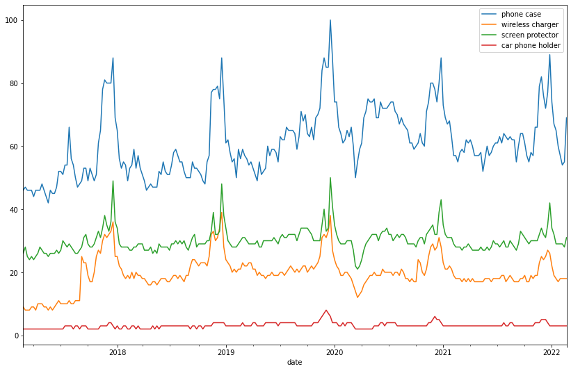
Now we’ll create a list of search terms we want to compare and analyse. Let’s pretend we’re an ecommerce retailer selling phone cases, wireless chargers, screen protectors, and car phone holders, and that we want to understand whether the market for these items is growing or declining, and where the peaks and troughs lie.
We’ll create a list called TERMS and will store the search terms we want to examine from Google Trends, and we’ll create a constant called FORECAST_WEEKS for later use that we’ll set to a 52 week period.
TERMS = ['phone case', 'wireless charger', 'screen protector', 'car phone holder']
FORECAST_WEEKS = 52
We’ll instantiate TrendReq() and define that we want searches for en-GB, then we’ll build a payload containing our TERMS and return a Pandas dataframe containing the search metrics for each term using pytrends.interest_over_time().
pt = TrendReq(hl='en-GB')
pt.build_payload(TERMS)
df = pt.interest_over_time()
df.plot(figsize=(14,9))
Reformat the data for the NeuralProphet model
Next, we’ll examine one specific search term and use NeuralProphet to create a time series forecast showing the growth or decline of the search volume for that term over the next FORECAST_WEEKS weeks. Since PyTrends can return partial data, we’ll use a filter to ensure we only get complete data points.
Then we’ll format the data for NeuralProphet by ensuring the date is renamed ds using the Pandas rename function and the target parameter we want to predict is stored in a column called y. If you don’t do this, NeuralProphet won’t run.
TARGET_TERM = 'phone case'

df = df[df['isPartial']==False].reset_index()
data = df.rename(columns={'date': 'ds', TARGET_TERM: 'y'})[['ds', 'y']]
data.tail()
| ds | y | |
|---|---|---|
| 255 | 2022-01-16 | 65 |
| 256 | 2022-01-23 | 60 |
| 257 | 2022-01-30 | 57 |
| 258 | 2022-02-06 | 54 |
| 259 | 2022-02-13 | 55 |
Create a NeuralProphet forecasting model
Now we can create the NeuralProphet model and fit it to our data. We’ll set the daily_seasonality argument to True, and then use the fit method to fit the model to our data.
model = NeuralProphet(daily_seasonality=True)
metrics = model.fit(data, freq="W")
INFO - (NP.utils.set_auto_seasonalities) - Disabling weekly seasonality. Run NeuralProphet with weekly_seasonality=True to override this.
INFO - (NP.config.set_auto_batch_epoch) - Auto-set batch_size to 16
INFO - (NP.config.set_auto_batch_epoch) - Auto-set epochs to 252


  0%|          | 0/221 [00:00<?, ?it/s]


INFO - (NP.utils_torch.lr_range_test) - lr-range-test results: steep: 4.02E-02, min: 5.62E-01


  0%|          | 0/221 [00:00<?, ?it/s]


INFO - (NP.utils_torch.lr_range_test) - lr-range-test results: steep: 3.03E-02, min: 6.18E-01


  0%|          | 0/221 [00:00<?, ?it/s]


INFO - (NP.utils_torch.lr_range_test) - lr-range-test results: steep: 3.33E-02, min: 3.86E-01
INFO - (NP.forecaster._init_train_loader) - lr-range-test selected learning rate: 3.44E-02
Epoch[252/252]: 100%|██████████| 252/252 [00:02<00:00, 84.48it/s, SmoothL1Loss=0.00488, MAE=2.73, RMSE=3.68, RegLoss=0]
Create a future dataframe
Next we’ll create a future dataframe containing the dates for the next 52 weeks. We’ll also tell NeuralProphet that we want to make historic predictions on the previous data.
future = model.make_future_dataframe(data, periods=FORECAST_WEEKS, n_historic_predictions=True)
future.head()
| ds | y | |
|---|---|---|
| 0 | 2017-02-26 | 46 |
| 1 | 2017-03-05 | 47 |
| 2 | 2017-03-12 | 46 |
| 3 | 2017-03-19 | 46 |
| 4 | 2017-03-26 | 46 |
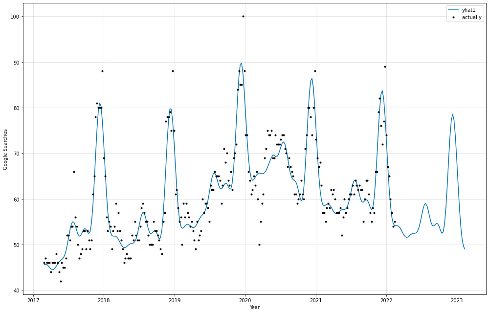
Create the time series forecast
Finally, we can use the predict method to create the time series forecast. We’ll pass in the future dataframe we created earlier, and assign the results to a Pandas dataframe called forecast. Then, we’ll plot the forecast using the plot() method.
forecast = model.predict(future)
ax = model.plot(forecast, ylabel='Google Searches', xlabel='Year', figsize=(14,9))
The blue line represents the forecast value, while the black dots represent the actual value recorded on each week shown in the Google Trends data. The forecast follows the general trend observed in the actual values without significant overfitting, suggesting that the forecast for the coming period should be a good indicator of what we might expect to see.
Matt Clarke, Wednesday, February 23, 2022


Other posts you might like

How to tune a LightGBMClassifier model with Optuna
The LightGBM model is a gradient boosting framework that uses tree-based learning algorithms, much like the popular XGBoost model. LightGBM supports both classification and regression tasks, and is known for...

How to create a customer retention model with XGBoost
Although all business know the importance of retaining customers, few companies are actually able to measure customer retention accurately, and fewer still can predict which ones will churn or be...
