How to use Recursive Feature Elimination in your models using RFECV

Picture by Tine Ivanic, Unsplash.

9 minutes to read

Something which often confuses non data scientists is that too many features can be a bad thing for a model. It does sound logical that including more features and data might make a model better. However, many features turn out to be uninformative and can actually mislead machine learning models and reduce their performance.

Therefore, one of the steps you’ll likely go through when building a larger model is a process aimed at taking out the irrelevant features that don’t add anything to improve the model’s performance. This process is known as feature selection and is commonly tackled using a technique called Recursive Feature Elimination or RFE.

Recursive Feature Elimination is quite a clever solution to the problem, I think. Recursion is the process of repeating a process multiple times. In the case of RFE, the process is that a separate model is trained and each time different features are taken away. While this process takes place, we observe the impact this has upon the model’s accuracy to determine the optimum set of features to use for the maximum results. Here’s how to use it.

Load the packages

For this project we’ll be using Pandas for data manipulation, Matplotlib for plotting, and a number of different packages from Scikit-Learn, including RFECV for the Recursive Feature Elimination. Load up the packages and install anything you don’t have by entering pip3 install package-name into your terminal.

import pandas as pd
import matplotlib.pyplot as plt
from sklearn.datasets import make_classification
from sklearn.model_selection import StratifiedKFold
from sklearn.feature_selection import RFECV
from sklearn.datasets import make_classification
from sklearn.tree import DecisionTreeClassifier

pd.set_option('max_columns', 6)

Create a high dimension data set

For this project we’ll create our own synthetic data set specifically engineered so it has a high number of dimensions. We’ll use the make_classification() method from Scikit-Learn to do this. We’ll define 1000 samples with 200 features, of which 6 will be informative and useful to the model, and 10 with be uninformative or redundant. We’ll make this a simple binary classification problem.

X, y = make_classification(n_samples=1000,
                           n_features=200,
                           n_informative=6,
                           n_redundant=10,
                           n_classes=2,
                           random_state=0
                          )

Once that’s created, we’ll save the resulting Numpy arrays to Pandas dataframes and then print out the shape of the dataframes and check to see how balanced the target variable is within the y data set by using the value_counts() function.

X = pd.DataFrame(X)
y = pd.Series(y)

print(X.shape, y.shape)

(1000, 200) (1000,)

y.value_counts()

0    504
1    496
dtype: int64

Fit a Recursive Feature Elimination model

Next we’ll use the RFECV() feature selection tool in Scikit-Learn to identify the optimum number of features to use in our model to obtain the highest accuracy score. To use this we pass in another Scikit-Learn classifier model to use as the estimator. I’ve used DecisionTreeClassifier().

As RFECV() also handles cross-validation, I’ve set this to use the StratifiedKFold() method and have selected 10 rounds, with accuracy used as my scoring metric. Once that’s set up, I’ve then fit it to my X and y data.

rfecv = RFECV(estimator=DecisionTreeClassifier(), 
              step=1, 
              cv=StratifiedKFold(10),
              scoring='accuracy')
rfecv.fit(X, y)

RFECV(cv=StratifiedKFold(n_splits=10, random_state=None, shuffle=False),
      estimator=DecisionTreeClassifier(), scoring='accuracy')

Examine the output

The rfecv object contains five attributes in its output: n_features_ contains the number of features selected via cross-validation; support_ contains a mask array of the selected features; ranking_ contains the feature ranking of the best features; grid_scores_ contains the cross-validation scores, and estimators_ is an object contain the estimator we used to reduce dimensionality, i.e. DecisionTreeClassifier(). If you print out the rfecv.n_features_ value you’ll see that this has correctly determined there are 5 informative features in the data.

print("Optimum number of features: %d" % rfecv.n_features_)

Optimum number of features: 6

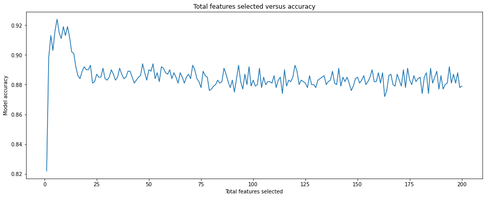
To visualise how the model’s performance drops off when you don’t reduce the number of features we can plot the number of features used in the model versus the model accuracy. As you can see, more features isn’t always better, and the model’s accuracy quickly drops off when uninformative features start racking up.

plt.figure( figsize=(16, 6))
plt.title('Total features selected versus accuracy')
plt.xlabel('Total features selected')
plt.ylabel('Model accuracy')
plt.plot(range(1, len(rfecv.grid_scores_) + 1), rfecv.grid_scores_)
plt.show()

png

Identifying the features RFE selected

As we saw above, the rfecv object contains some hidden data attributes that we can extract to identify which features the DecisionTreeClassifier() identified from our data set as those which were informative. To extract these we’ll create a dataframe, loop through the data and append a new row to the dataframe containing the feature index number, the support level and the ranking. To extract only the informative ones we can then use df_features[df_features['support']==True].

df_features = pd.DataFrame(columns = ['feature', 'support', 'ranking'])

for i in range(X.shape[1]):
    row = {'feature': i, 'support': rfecv.support_[i], 'ranking': rfecv.ranking_[i]}
    df_features = df_features.append(row, ignore_index=True)
    
df_features.sort_values(by='ranking').head(10)

	feature	support	ranking
199	199	True	1
86	86	True	1
88	88	True	1
151	151	True	1
104	104	True	1
161	161	True	1
143	143	False	2
79	79	False	3
64	64	False	4
40	40	False	5

df_features[df_features['support']==True]

	feature	support	ranking
86	86	True	1
88	88	True	1
104	104	True	1
151	151	True	1
161	161	True	1
199	199	True	1

Finally, to extract the selected features and use them as the model features in X you can run the get_support() function and pass in an argument of 1 to return all of the items with support.

selected_features = rfecv.get_support(1)
X = df[df.columns[selected_features]]

Matt Clarke, Saturday, March 06, 2021

Matt Clarke Matt is an Ecommerce and Marketing Director who uses data science to help in his work. Matt has a Master's degree in Internet Retailing (plus two other Master's degrees in different fields) and specialises in the technical side of ecommerce and marketing.