How to use SMOTE for imbalanced classification
SMOTE, the Synthetic Minority Oversampling Technique, is one of the best ways to handle imbalanced classification modeling tasks. Here's how to use it.

Imbalanced classification problems, such as the detection of fraudulent card payments, represent a significant challenge for machine learning models. When the target class, such as fraudulent transactions, makes up such a tiny percentage of the total data set, it can be tricky for the model to identify them and the model may over-predict the majority class because the “decision boundary” is unclear.
There are several techniques you can use to improve the performance of your machine learning models, most commonly using either under-sampling or over-sampling. Under-sampling effectively discards data on the majority class (i.e. non-fraudulent transactions) until it’s in balance with the minority class (i.e. fraudulent transactions).
The downside of under-sampling is that the model discards potentially useful data and is trained on a much smaller data set.
Over-sampling does the opposite and scales up the volume of the minority class data by duplicating it, until it’s equal to that of the majority class. The most popular way of doing this is via a clever technique known as SMOTE.
What is SMOTE?
SMOTE stands for Synthetic Minority Oversampling Technique. As the name suggests, this takes the minority class (i.e. fraudulent transactions, terrorists, or trustworthy politicians) and adds new examples to the data set until the quantity of the two classes are equal. However, it doesn’t just do this by duplicating the data already present. Instead, it creates new synthetic data containing plausible values that are close to the “feature space” of the minority class using data augmentation.
While the SMOTE technique is often used as-is, the authors of the original paper actually recommend that it’s used in conjunction with under-sampling.
Using the under-sample and over-sample approach, the aim is to randomly under-sample the majority class to reduce the number of values - many of which will not add very much to the performance of the model - and use SMOTE to over-sample the minority. Let’s take a look at how it’s done.
Load the packages
We need quite a few packages for this project. You may have most of these already installed, but if not, they can each be installed via the Python Package Index or PyPi using the command pip3 install package-name. You can do this from within a Jupyter notebook by entering !pip3 install package-name and then executing the code cell.
import pandas as pd
import numpy as np
import time
import matplotlib.pyplot as plt
from imblearn.over_sampling import SMOTE
from imblearn.over_sampling import BorderlineSMOTE
from imblearn.under_sampling import RandomUnderSampler
from xgboost import XGBClassifier
from lightgbm import LGBMClassifier
from sklearn.dummy import DummyClassifier
from sklearn.neighbors import KNeighborsClassifier
from sklearn.tree import DecisionTreeClassifier
from sklearn.ensemble import RandomForestClassifier
from sklearn.ensemble import AdaBoostClassifier
from sklearn.ensemble import GradientBoostingClassifier
from sklearn.naive_bayes import GaussianNB
from sklearn.linear_model import LogisticRegression
from sklearn.model_selection import RepeatedStratifiedKFold
from sklearn.model_selection import cross_val_score
from sklearn.model_selection import train_test_split
from sklearn.metrics import classification_report
from sklearn.metrics import confusion_matrix
from sklearn.metrics import f1_score
from sklearn.metrics import accuracy_score
from sklearn.metrics import roc_auc_score
from sklearn.metrics import precision_score
from sklearn.metrics import recall_score
from sklearn.metrics import average_precision_score
from sklearn.metrics import precision_recall_curve
from sklearn.metrics import make_scorer
Load the data
One of the best datasets for honing your imbalanced classification skills is the Credit Card Fraud Detection data set. This anonymised data set contains 284K transactions from a two day period, during which 492 or 0.173% of orders were fraudulent.
After downloading the data set from Kaggle, load it up into Pandas and convert the column names to lower case. To help all the columns fit on the page, I’ve transposed the orientation of the data using .T. My separate exploratory data analysis showed that the time column contains a timestamp which wasn’t correlated with the target and appears to leak data, so I’m dropping this one from the dataframe before proceeding.
df = pd.read_csv('creditcard.csv')
df.columns = map(str.lower, df.columns)
df = df.drop('time', axis=1)
df.head().T
| 0 | 1 | 2 | 3 | 4 | |
|---|---|---|---|---|---|
| v1 | -1.359807 | 1.191857 | -1.358354 | -0.966272 | -1.158233 |
| v2 | -0.072781 | 0.266151 | -1.340163 | -0.185226 | 0.877737 |
| v3 | 2.536347 | 0.166480 | 1.773209 | 1.792993 | 1.548718 |
| v4 | 1.378155 | 0.448154 | 0.379780 | -0.863291 | 0.403034 |
| v5 | -0.338321 | 0.060018 | -0.503198 | -0.010309 | -0.407193 |
| v6 | 0.462388 | -0.082361 | 1.800499 | 1.247203 | 0.095921 |
| v7 | 0.239599 | -0.078803 | 0.791461 | 0.237609 | 0.592941 |
| v8 | 0.098698 | 0.085102 | 0.247676 | 0.377436 | -0.270533 |
| v9 | 0.363787 | -0.255425 | -1.514654 | -1.387024 | 0.817739 |
| v10 | 0.090794 | -0.166974 | 0.207643 | -0.054952 | 0.753074 |
| v11 | -0.551600 | 1.612727 | 0.624501 | -0.226487 | -0.822843 |
| v12 | -0.617801 | 1.065235 | 0.066084 | 0.178228 | 0.538196 |
| v13 | -0.991390 | 0.489095 | 0.717293 | 0.507757 | 1.345852 |
| v14 | -0.311169 | -0.143772 | -0.165946 | -0.287924 | -1.119670 |
| v15 | 1.468177 | 0.635558 | 2.345865 | -0.631418 | 0.175121 |
| v16 | -0.470401 | 0.463917 | -2.890083 | -1.059647 | -0.451449 |
| v17 | 0.207971 | -0.114805 | 1.109969 | -0.684093 | -0.237033 |
| v18 | 0.025791 | -0.183361 | -0.121359 | 1.965775 | -0.038195 |
| v19 | 0.403993 | -0.145783 | -2.261857 | -1.232622 | 0.803487 |
| v20 | 0.251412 | -0.069083 | 0.524980 | -0.208038 | 0.408542 |
| v21 | -0.018307 | -0.225775 | 0.247998 | -0.108300 | -0.009431 |
| v22 | 0.277838 | -0.638672 | 0.771679 | 0.005274 | 0.798278 |
| v23 | -0.110474 | 0.101288 | 0.909412 | -0.190321 | -0.137458 |
| v24 | 0.066928 | -0.339846 | -0.689281 | -1.175575 | 0.141267 |
| v25 | 0.128539 | 0.167170 | -0.327642 | 0.647376 | -0.206010 |
| v26 | -0.189115 | 0.125895 | -0.139097 | -0.221929 | 0.502292 |
| v27 | 0.133558 | -0.008983 | -0.055353 | 0.062723 | 0.219422 |
| v28 | -0.021053 | 0.014724 | -0.059752 | 0.061458 | 0.215153 |
| amount | 149.620000 | 2.690000 | 378.660000 | 123.500000 | 69.990000 |
| class | 0.000000 | 0.000000 | 0.000000 | 0.000000 | 0.000000 |
Examine the class imbalance
To examine the class imbalance of a data set you can use the Pandas value_counts() function on the target
column of the dataframe, which is called class on this data set. As you can see, we have 284,315 non-fraudulent transactions in class 0 and 492 fraudulent transactions in class 1. This will represent a massive challenge for most models, since they’l favour the dominant class and predict that the very vast majority of orders are non-fraudulent.
df['class'].value_counts()
0    284315
1       492
Name: class, dtype: int64
(492/284315)*100
0.17304750013189596
100-(492/284315)*100
99.8269524998681
By grouping by the class column and then creating an agg() we can calculate the costs of fraud. The data set is based on a two day period, in which there were 492 fraudulent transactions potentially generating £60,127.97 in lost revenue. Using a naiive extrapolation, as we don’t have the full data set, this is equivalent to £30,063.98 per day. Therefore, we’re looking at annual fraud costs of around £10,973,354.
df.groupby('class').agg(
    transactions=('class', 'count'),
    total_revenue=('amount', 'sum'),
).round(2)
| transactions | total_revenue | |
|---|---|---|
| class | ||
| 0 | 284315 | 25102462.04 |
| 1 | 492 | 60127.97 |
Examine correlation with the target
Next, we’ll take a quick look at the Pearson correlation coefficients of each column compared to the target class. Although we don’t know what the features relate to, because the bank has hidden these details from us so we can’t exploit them to commit fraud ourselves, we can see that some of them have moderate correlations with fraudulent or non-fraudulent transactions in both the negative and positive direction. For example, v11 has the strongest positive correlation and v17 has the strongest negative correlation. There are certainly some indicators in here to guide our model.
df[df.columns[1:]].corr()['class'][:].sort_values(ascending=False)
class     1.000000
v11       0.154876
v4        0.133447
v2        0.091289
v21       0.040413
v19       0.034783
v20       0.020090
v8        0.019875
v27       0.017580
v28       0.009536
amount    0.005632
v26       0.004455
v25       0.003308
v22       0.000805
v23      -0.002685
v15      -0.004223
v13      -0.004570
v24      -0.007221
v6       -0.043643
v5       -0.094974
v9       -0.097733
v18      -0.111485
v7       -0.187257
v3       -0.192961
v16      -0.196539
v10      -0.216883
v12      -0.260593
v14      -0.302544
v17      -0.326481
Name: class, dtype: float64
Split the data
We’ll define all of the fields (minus the time column we dropped earlier and the target class) to the X dataframe and the class values to the y dataframe. Next we need to split our data into the train and test datasets. We’ll use the train data set to train the model and we’ll hold back the test data set. Once the model has been trained, we can then verify it’s performance by using it to predict the outcome from the test data set, for which it has not previously seen the answers. The train_test_split() function allows you to perform this step.
It’s common to set the test_size to a value of 0.2 to 0.33, which assigns 20% or 33% to the test group. The random_state value ensures reproducibility, shuffle, ensures the data are jumbled up, just in case all the fraudulent orders sit together within the data, and stratify ensures we have the same percentage of fraudulent orders in both the train and test datasets.
X = df.drop('class', axis=1)
y = df['class']
X_train, X_test, y_train, y_test = train_test_split(X, y,
                                                    test_size=0.3,
                                                    random_state=0,
                                                    shuffle=True,
                                                    stratify=y)
Selecting the right performance metric
Before we get started, we need to figure out which is the best metric to use to measure the performance of our model. This data set is extremely imbalanced, so you can’t use a metric like accuracy. For example, if a model predicted the minority class every time, it would still reach 99.826% accuracy, which seems good, but it completely fails to detect any fraudulent orders, defeating the object of the task entirely.
The area under the Receiver Operating Characteristic curve or AUROC (or AUC/ROC) is commonly used to evaluate classification models. It’s much better to use than accuracy on imbalanced data because it uses the true positive rate and the true negative rate. However, it’s not always ideal to use on extremely imbalanced datasets in which you aim most to identify the positive class - i.e. people placing fraudulent orders, terrorists, or people suffering from some nasty disease.
For example, check out the results below, based on three models trained on this data set. Model 1 has an AUROC of 0.882 and identifies 113 fraudulent orders (tp) and misses 35 (fn), while incorrectly flagging 6 as fraudulent (fp). Model 2 performs better, with an AUROC of 0.918, and correctly identifies 124 fraudulent orders (tp), misses 24 (fn), while incorrectly flagging 27 as fraudulent (fp). While Model 3 gains an AUROC of 0.933, based on 134 correctly flagged fraudulent orders (tp), a lower number of false negatives at 14, but with a massive 3339 non-fraudulent orders incorrectly flagged as fradulent.
| model | tp | tn | fp | fn | correct | incorrect | accuracy | precision | recall | f1 | roc_auc | |
|---|---|---|---|---|---|---|---|---|---|---|---|---|
| 0 | Model 1 | 113 | 85289 | 6 | 35 | 85402 | 41 | 1.000000 | 0.950000 | 0.764000 | 0.846000 | 0.882000 |
| 1 | Model 2 | 124 | 85268 | 27 | 24 | 85392 | 51 | 0.999403 | 0.821192 | 0.837838 | 0.829431 | 0.918761 |
| 2 | Model 3 | 134 | 81956 | 3339 | 14 | 82090 | 3353 | 0.960757 | 0.038583 | 0.905405 | 0.074013 | 0.933129 |
Clearly, although it’s good that Model 3 gets more right, it wouldn’t be a great customer experience for thousands of customers to have their orders incorrectly blocked for being fraudulent when they weren’t, just as it wouldn’t be ideal detaining innocent people believed to be terrorists, or incorrectly telling patients they had life threatening diseases when they were fine… Clearly, AUROC isn’t ideal for this data set.
AUPRC
The metric favoured in such situations is called AUPRC, or area under the precision and recall curve. AUPRC provides a better way for measuring model performance in those situations where you care most about finding the positive outcomes of a minority class, such as fraudulent transactions, terrorists, or diseases. It’s much more useful to us than the area under the receiver operating characteristic or AUROC (ROC/AUC) as it shows the trade off between precision and recall and it ignores true negatives.
AUPRC is much harder to interpret than AUROC because the baseline differs on every data set. A baseline random classifier will give an AUROC of 0.5, but for AUPRC the baseline is equal to the fraction of positives. Therefore, on a data set with 10% positive examples, you get a baseline AUPRC of 0.1, so scoring 0.2 would be a good score, and 0.4 excellent. On our data set, we have 492 positive examples out of 284,807 in total, so our baseline AUROC is just 0.001727. A good model could therefore have a seemingly low score.
AUPRC is a bit tricky to calculate, so most people instead calculate average precision, which is very close. Precision is the ratio of true positives over the true positives + true negatives, i.e. precision = tp / (tp + fp). However, I’m not entirely convinced it’s perfect for this application, so you would be wise to check your own results.
Fit a baseline model
Firstly, to show what happens when you fit a classification model to an extremely imbalanced data set like this one we will fit some baseline models and examine how they perform. One of these is a DummyClassifier() models set to predict the most_frequent value. This should say all the orders are non-fraudulent, thus giving us 99.8% accuracy, but completely failing to spot any fraudulent orders. The others are a range of popular classification models, including random forest, decision tree, Gaussian Naiive Bayes, K nearest neighbours or KNN, logistic regression, and several gradient boosting models.
classifiers = {
    "DummyClassifier_most_frequent": DummyClassifier(strategy='most_frequent', random_state=0),
    "LogisticRegression": LogisticRegression(solver = 'lbfgs', max_iter=1000),
    "LGBMClassifier": LGBMClassifier(),
    "XGBClassifier": XGBClassifier(),
    "KNeighborsClassifier": KNeighborsClassifier(3),
    "DecisionTreeClassifier": DecisionTreeClassifier(),
    "RandomForestClassifier": RandomForestClassifier(),
    "AdaBoostClassifier": AdaBoostClassifier(),
    "GradientBoostingClassifier": GradientBoostingClassifier(),
    "GaussianNB": GaussianNB(),
}
We will now loop over each of the models in the above dictionary, fit the model to the training data set, and define a repeated stratified K fold cross validation (this ensures each fold contains equal proportions of the positive class). We’ll create a custom scorer using make_scorer() to calculate the average precision in the cross validation for each model and then place the results into a Pandas dataframe. As this is quite a large data set, you may want to go away and have a cup of tea or go for a walk while this runs. Even on my powerful workstation this took a fairly long time to complete.
df_models = pd.DataFrame(columns=['model', 'run_time', 'avg_pre', 'avg_pre_std'])

for key in classifiers:

    print('*',key)

    start_time = time.time()

    classifier = classifiers[key]
    model = classifier.fit(X_train, y_train)
    cv = RepeatedStratifiedKFold(n_splits=10, n_repeats=5, random_state=1)
    scorer = make_scorer(average_precision_score)
    cv_scores = cross_val_score(model, X_test, y_test, cv=5, scoring=scorer)
    y_pred = model.predict(X_test)

    row = {'model': key,
           'run_time': format(round((time.time() - start_time)/60,2)),
           'avg_pre': cv_scores.mean(),
           'avg_pre_std': cv_scores.std(),
    }

    df_models = df_models.append(row, ignore_index=True)
* DummyClassifier_most_frequent
* LogisticRegression
* LGBMClassifier
* XGBClassifier
* KNeighborsClassifier
* DecisionTreeClassifier
* RandomForestClassifier
* AdaBoostClassifier
* GradientBoostingClassifier
* GaussianNB
The DummyClassifier set to most_frequent achieved a ROC/AUC score of 0.5 and an average precision of 0.001732, as it predicted every transaction to be non-fraudulent. This is our baseline score (it’s effectively the AUPRC). The stratified approach was slightly better, but still barely any better than random guessing. The other models differ quite widely in their scores. The best model was XGBoost, in which it achieved an average precision of 0.664627.
df_models.head(10).sort_values(by='avg_pre')
| model | run_time | avg_pre | avg_pre_std | |
|---|---|---|---|---|
| 0 | DummyClassifier_most_frequent | 0.0 | 0.001732 | 0.000029 |
| 9 | GaussianNB | 0.0 | 0.052575 | 0.012273 |
| 2 | LGBMClassifier | 0.04 | 0.074877 | 0.041033 |
| 8 | GradientBoostingClassifier | 8.62 | 0.298909 | 0.128801 |
| 5 | DecisionTreeClassifier | 0.45 | 0.430833 | 0.092404 |
| 4 | KNeighborsClassifier | 1.12 | 0.488499 | 0.088547 |
| 1 | LogisticRegression | 0.4 | 0.491425 | 0.067003 |
| 7 | AdaBoostClassifier | 1.67 | 0.532776 | 0.054281 |
| 6 | RandomForestClassifier | 4.55 | 0.657685 | 0.085107 |
| 3 | XGBClassifier | 0.22 | 0.664627 | 0.090546 |
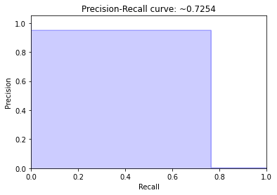
If we re-run the XGBClassifier and calculate some metrics we can see how it performs on the test data. The ROC/AUC score here was 0.88 and the average precision was 0.725. It correctly predicted 85402 of the non-fraudulent transactions and 113 of the fraudulent transactions, but misidentified 6 non-fraudulent orders as fraudulent and, worse, missed 35 fraduluent orders.
df_result = pd.DataFrame(columns=['model', 'tp', 'tn', 'fp', 'fn', 'correct', 'incorrect',
                                  'accuracy', 'precision', 'recall', 'f1', 'roc_auc','avg_pre'])

classifier = XGBClassifier(random_state=123)
model = classifier.fit(X_train, y_train)
y_pred = model.predict(X_test)

tn, fp, fn, tp = confusion_matrix(y_test, y_pred).ravel()
accuracy = accuracy_score(y_test, y_pred)
precision = precision_score(y_test, y_pred)
recall = recall_score(y_test, y_pred)
f1 = f1_score(y_test, y_pred)
roc_auc = roc_auc_score(y_test, y_pred)
avg_precision = average_precision_score(y_test, y_pred)

row = {'model': 'XGBClassifier without SMOTE',
        'tp': tp,
        'tn': tn,
        'fp': fp,
        'fn': fn,
        'correct': tp+tn,
        'incorrect': fp+fn,
        'accuracy': round(accuracy,3),
        'precision': round(precision,3),
        'recall': round(recall,3),
        'f1': round(f1,3),
        'roc_auc': round(roc_auc,3),
        'avg_pre': round(avg_precision,3),
    }

df_result = df_result.append(row, ignore_index=True)
df_result.head()
| model | tp | tn | fp | fn | correct | incorrect | accuracy | precision | recall | f1 | roc_auc | avg_pre | |
|---|---|---|---|---|---|---|---|---|---|---|---|---|---|
| 0 | XGBClassifier without SMOTE | 113 | 85289 | 6 | 35 | 85402 | 41 | 1.0 | 0.95 | 0.764 | 0.846 | 0.882 | 0.725 |
avg_precision = average_precision_score(y_test, y_pred)
precision, recall, _ = precision_recall_curve(y_test, y_pred)

plt.step(recall, precision, color='b', alpha=0.2, where='post')
plt.fill_between(recall, precision, step='post', alpha=0.2, color='b')

plt.xlabel('Recall')
plt.ylabel('Precision')
plt.ylim([0.0, 1.05])
plt.xlim([0.0, 1.0])
plt.title('Precision-Recall curve: ~{0:0.4f}'.format(avg_precision))
Text(0.5, 1.0, 'Precision-Recall curve: ~0.7254')
Fit a model using SMOTE
Next, we’ll use the common technique of simply applying SMOTE to the data to over-sample the minority class, without applying any under-sampling. To do this we can use the Imbalanced Learning package imblearn which works with Scikit-Learn’s packages to apply the SMOTE algorithm and generate realistic synthetic data, rather than simply duplicating it. To show the whole process, we’ll re-split the test and training data first.
X_train, X_test, y_train, y_test = train_test_split(X, y,
                                                    test_size=0.3,
                                                    random_state=0,
                                                    shuffle=True,
                                                    stratify=y)
Next we will instantiate SMOTE() and then run the fit_sample() function on the X_train and y_train data. It’s important not to run this on the whole X and y datasets. The test data you pass in needs to reflect how it will appear in the real world, where the classes can’t be balanced. You can run value_counts() to check the classes are balanced afterwards. As you can see, we now have 199020 records in each class.
oversampled = SMOTE(random_state=0)
X_train_smote, y_train_smote = oversampled.fit_sample(X_train, y_train)
y_train_smote.value_counts()
1    199020
0    199020
Name: class, dtype: int64
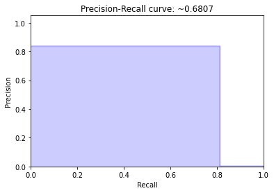
Now we will re-train the XGBClassifier on the oversampled data, then we’ll just repeat the above process and calculate the scores for predictions against the test data set. This pushes the ROC/AUC score up from 0.88 to 0.92, but the average precision falls. However, checking the results, shows we actually performed better using this approach.
classifier = XGBClassifier(random_state=222)
model = classifier.fit(X_train_smote, y_train_smote)
y_pred_smote = model.predict(X_test)
tn, fp, fn, tp = confusion_matrix(y_test, y_pred_smote).ravel()
accuracy = accuracy_score(y_test, y_pred_smote)
precision = precision_score(y_test, y_pred_smote)
recall = recall_score(y_test, y_pred_smote)
f1 = f1_score(y_test, y_pred_smote)
roc_auc = roc_auc_score(y_test, y_pred_smote)
avg_precision = average_precision_score(y_test, y_pred_smote)

row = {'model': 'XGBClassifier with SMOTE',
        'tp': tp,
        'tn': tn,
        'fp': fp,
        'fn': fn,
        'correct': tp+tn,
        'incorrect': fp+fn,
        'accuracy': accuracy,
        'precision': precision,
        'recall': recall,
        'f1': f1,
        'roc_auc': roc_auc,
        'avg_pre': round(avg_precision,3),
    }
The model which uses SMOTE correctly identified 122 fraudulent orders instead of 113 and incorrectly missed 26 fraudulent orders instead of 35, which was at the expensive of an increase in the number of false positives, which increased from 6 to 25. However, in terms of the cost, incorrectly predicting fraud may not cost as much as missing it.
df_result = df_result.append(row, ignore_index=True)
df_result.head()
| model | tp | tn | fp | fn | correct | incorrect | accuracy | precision | recall | f1 | roc_auc | avg_pre | |
|---|---|---|---|---|---|---|---|---|---|---|---|---|---|
| 0 | XGBClassifier without SMOTE | 113 | 85289 | 6 | 35 | 85402 | 41 | 1.000000 | 0.950000 | 0.764000 | 0.846000 | 0.882000 | 0.725 |
| 1 | XGBClassifier with SMOTE | 120 | 85272 | 23 | 28 | 85392 | 51 | 0.999403 | 0.839161 | 0.810811 | 0.824742 | 0.905271 | 0.681 |
avg_precision = average_precision_score(y_test, y_pred_smote)
precision, recall, _ = precision_recall_curve(y_test, y_pred_smote)

plt.step(recall, precision, color='b', alpha=0.2, where='post')
plt.fill_between(recall, precision, step='post', alpha=0.2, color='b')

plt.xlabel('Recall')
plt.ylabel('Precision')
plt.ylim([0.0, 1.05])
plt.xlim([0.0, 1.0])
plt.title('Precision-Recall curve: ~{0:0.4f}'.format(avg_precision))
Text(0.5, 1.0, 'Precision-Recall curve: ~0.6807')
Using under-sampling and SMOTE over-sampling
Next we’ll use a mixture of under-sampling and over-sampling to see if we can improve the scores. This approach takes much more trial and error, so I’d suggest creating a loop to go over a range of values to identify the settings which provide the best results. Firstly, we’ll check the value_counts() on our class data from the then we’ll re-split our data using train_test_split().
y.value_counts()
0    284315
1       492
Name: class, dtype: int64
X_train, X_test, y_train, y_test = train_test_split(X, y,
                                                    test_size=0.3,
                                                    random_state=0,
                                                    shuffle=True,
                                                    stratify=y)
We’ll now use SMOTE to oversample the minority class so it represents 40% of the total. You’ll want to try a range of different values here to see what works best. I’ve also added in the k_neighbors argument to define the number of neighbours to use when creating the data. Again, try different values to see what happens on your data set.
oversampled = SMOTE(sampling_strategy=0.6,
                    random_state=0,
                    k_neighbors=4)
X_train_smote, y_train_smote = oversampled.fit_sample(X_train, y_train)
y_train_smote.value_counts()
0    199020
1    119412
Name: class, dtype: int64
Now we’ll take our oversampled data and undersample it using RandomUnderSampler. After some fiddling, I found I got better results by using a 0.7 sampling strategy, which put 170,588 transactions in the minority class and 119,412 in the majority class.
undersampled = RandomUnderSampler(sampling_strategy=0.7, random_state=0)
X_train_final, y_train_final = undersampled.fit_sample(X_train_smote, y_train_smote)
y_train_final.value_counts()
0    170588
1    119412
Name: class, dtype: int64
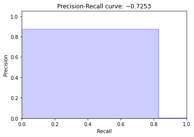
Finally, I’ve created a new XGBoost classifier and trained it on the oversampled and undersampled data, and then calculated the scores and appended them to the dataframe containing the results of the models.
classifier = XGBClassifier(random_state=222)
model = classifier.fit(X_train_final, y_train_final)
y_pred_smote = model.predict(X_test)
tn, fp, fn, tp = confusion_matrix(y_test, y_pred_smote).ravel()
accuracy = accuracy_score(y_test, y_pred_smote)
precision = precision_score(y_test, y_pred_smote)
recall = recall_score(y_test, y_pred_smote)
f1 = f1_score(y_test, y_pred_smote)
roc_auc = roc_auc_score(y_test, y_pred_smote)
avg_precision = average_precision_score(y_test, y_pred_smote)

row = {'model': 'XGBClassifier with under/over',
        'tp': tp,
        'tn': tn,
        'fp': fp,
        'fn': fn,
        'correct': tp+tn,
        'incorrect': fp+fn,
        'accuracy': accuracy,
        'precision': precision,
        'recall': recall,
        'f1': f1,
        'roc_auc': roc_auc,
        'avg_pre': round(avg_precision,3),
    }
df_result = df_result.append(row, ignore_index=True)
df_result.tail(20)
| model | tp | tn | fp | fn | correct | incorrect | accuracy | precision | recall | f1 | roc_auc | avg_pre | |
|---|---|---|---|---|---|---|---|---|---|---|---|---|---|
| 0 | XGBClassifier without SMOTE | 113 | 85289 | 6 | 35 | 85402 | 41 | 1.000000 | 0.950000 | 0.764000 | 0.846000 | 0.882000 | 0.725 |
| 1 | XGBClassifier with SMOTE | 120 | 85272 | 23 | 28 | 85392 | 51 | 0.999403 | 0.839161 | 0.810811 | 0.824742 | 0.905271 | 0.681 |
| 2 | XGBClassifier with under/over | 123 | 85277 | 18 | 25 | 85400 | 43 | 0.999497 | 0.872340 | 0.831081 | 0.851211 | 0.915435 | 0.725 |
avg_precision = average_precision_score(y_test, y_pred_smote)
precision, recall, _ = precision_recall_curve(y_test, y_pred_smote)

plt.step(recall, precision, color='b', alpha=0.2, where='post')
plt.fill_between(recall, precision, step='post', alpha=0.2, color='b')

plt.xlabel('Recall')
plt.ylabel('Precision')
plt.ylim([0.0, 1.05])
plt.xlim([0.0, 1.0])
plt.title('Precision-Recall curve: ~{0:0.4f}'.format(avg_precision))
Text(0.5, 1.0, 'Precision-Recall curve: ~0.7253')
Borderline SMOTE
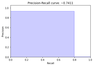
There are quite a few related techniques you can apply that are effectively modifications of the regular SMOTE technique. One of these is called Borderline SMOTE. Internally, Borderline SMOTE uses a Support Vector Machine model (SVM) to calculate the decision boundary, compared to the K nearest neighbours (KNN) model used in regular SMOTE. The process for creating the model is that same as above. We’re just replacing SMOTE() with BorderlineSMOTE().
X_train, X_test, y_train, y_test = train_test_split(X, y,
                                                    test_size=0.3,
                                                    random_state=0,
                                                    shuffle=True,
                                                    stratify=y)
oversampled = BorderlineSMOTE(random_state=0)
X_train_smote, y_train_smote = oversampled.fit_sample(X_train, y_train)
y_train_smote.value_counts()
1    199020
0    199020
Name: class, dtype: int64
classifier = XGBClassifier(random_state=222)
model = classifier.fit(X_train_smote, y_train_smote)
y_pred_smote = model.predict(X_test)
tn, fp, fn, tp = confusion_matrix(y_test, y_pred_smote).ravel()
accuracy = accuracy_score(y_test, y_pred_smote)
precision = precision_score(y_test, y_pred_smote)
recall = recall_score(y_test, y_pred_smote)
f1 = f1_score(y_test, y_pred_smote)
roc_auc = roc_auc_score(y_test, y_pred_smote)
avg_precision = average_precision_score(y_test, y_pred_smote)

row = {'model': 'XGBClassifier with Borderline SMOTE',
        'tp': tp,
        'tn': tn,
        'fp': fp,
        'fn': fn,
        'correct': tp+tn,
        'incorrect': fp+fn,
        'accuracy': accuracy,
        'precision': precision,
        'recall': recall,
        'f1': f1,
        'roc_auc': roc_auc,
        'avg_pre': round(avg_precision,3),
    }
The Borderline SMOTE model sees our average precision score increase but our AUROC fall and the model detects fewer true positives. It’s an improvement over the original model, but could still benefit from some tweaking to improve performance.
df_result = df_result.append(row, ignore_index=True)
df_result.head()
| model | tp | tn | fp | fn | correct | incorrect | accuracy | precision | recall | f1 | roc_auc | avg_pre | |
|---|---|---|---|---|---|---|---|---|---|---|---|---|---|
| 0 | XGBClassifier without SMOTE | 113 | 85289 | 6 | 35 | 85402 | 41 | 1.000000 | 0.950000 | 0.764000 | 0.846000 | 0.882000 | 0.725 |
| 1 | XGBClassifier with SMOTE | 120 | 85272 | 23 | 28 | 85392 | 51 | 0.999403 | 0.839161 | 0.810811 | 0.824742 | 0.905271 | 0.681 |
| 2 | XGBClassifier with under/over | 123 | 85277 | 18 | 25 | 85400 | 43 | 0.999497 | 0.872340 | 0.831081 | 0.851211 | 0.915435 | 0.725 |
| 3 | XGBClassifier with Borderline SMOTE | 118 | 85286 | 9 | 30 | 85404 | 39 | 0.999544 | 0.929134 | 0.797297 | 0.858182 | 0.898596 | 0.741 |
avg_precision = average_precision_score(y_test, y_pred_smote)
precision, recall, _ = precision_recall_curve(y_test, y_pred_smote)

plt.step(recall, precision, color='b', alpha=0.2, where='post')
plt.fill_between(recall, precision, step='post', alpha=0.2, color='b')

plt.xlabel('Recall')
plt.ylabel('Precision')
plt.ylim([0.0, 1.05])
plt.xlim([0.0, 1.0])
plt.title('Precision-Recall curve: ~{0:0.4f}'.format(avg_precision))
Text(0.5, 1.0, 'Precision-Recall curve: ~0.7411')
The end results…
Our best model, the XGBClassifier we used with both SMOTE and under-sampling, correctly identified 123 of the 148 fraudulent orders from within the data set of 284K total orders, while only incorrectly flagging 18 orders as fraud when they were non-fraudulent.
Based on an average value of £124.75 per fraudulent order, our model saved the bank around £15,344 per day, and about £5.6 million per year!
There’s still more we could do here, of course. We didn’t try feature engineering, remove outliers, or tune model hyper-parameters, or the settings used for SMOTE’s internal KNN model, so there’s room to get further improvement if you put in the time.
The trickiest bit seems to be finding the right metric to judge performance, as both ROC/AUC and average precision seem to have pros and cons. Perhaps a cost-based metric would work well? If you have any ideas on the best approach, please let me know in the comments.
Further reading
-
Brownlow, J (2020) - SMOTE for imbalanced classification with Python, Machine Learning Mastery.
-
Draelos, R (2019) - Measuring Performance: AUPRC and Average Precision, Glass Box Machine Learning and Medicine.
Matt Clarke, Saturday, March 06, 2021


Other posts you might like

How to tune a LightGBMClassifier model with Optuna
The LightGBM model is a gradient boosting framework that uses tree-based learning algorithms, much like the popular XGBoost model. LightGBM supports both classification and regression tasks, and is known for...

How to create a customer retention model with XGBoost
Although all business know the importance of retaining customers, few companies are actually able to measure customer retention accurately, and fewer still can predict which ones will churn or be...
