How to create ecommerce sales forecasts using Prophet
Creating accurate ecommerce time series forecasts using models such as ARIMA can be tricky. The Prophet forecasting model makes things much easier.

Time series forecasting models are notoriously tricky to master, especially in ecommerce, where you have seasonality, the weather, marketing promotions, and holidays to consider. Not to mention pandemics.
For many years, the standard tools used for time series forecasting have been the Auto-regressive Moving Average model (ARIMA) and its derivatives, such as SARIMA, and the more complex neural network Long Short Term Memory (LSTM) model.
Neither of them has a reputation for simplicity and producing quality forecasts with them takes considerable skill and experience. This is where the Prophet model comes in.
Prophet was developed by engineers at Facebook and open sourced. It’s used by Facebook themselves for producing reliable forecasts and they found it “better than any other approach in the majority of cases.”
Prophet is also pretty quick, can be fitted to data quickly, and can be run in parallel across multiple CPU cores. It’s written in Stan, a state-of-the-art platform for statistical modeling which is popular particularly for Bayesian inference and uses TensorFlow for its back-end. Prophet lets you fit time series forecasting models in seconds or minutes and allows you to tune them to handle business-specific holidays and seasonality.
Let’s take a look at how we can use Prophet to create some time series forecasting models to predict future traffic and revenue for an ecommerce website.
Set up your environment
As Prophet has specific package requirements, I’d recommend that you install it within a containerised environment using Docker. This will ensure it works correctly and doesn’t impact any other applications you have installed. You can follow this guide to see how that’s done.
Install the packages
For this project we’ll be working within a Jupyter notebook, so start your Docker container, fire up Jupyter, open a new notebook and run the commands below. As well as the usual pandas and numpy, we’ll be using itertools to handle some looping stuff, and a whole range of different modules from the fbprophet package. These handle various things, from creating the models, to plotting the output and measuring model performance.
import pandas as pd
import numpy as np
import itertools

from fbprophet import Prophet
from fbprophet.plot import plot_plotly
from fbprophet.plot import plot_components_plotly
from fbprophet.plot import add_changepoints_to_plot
from fbprophet.plot import plot_yearly
from fbprophet.plot import plot_cross_validation_metric
from fbprophet.diagnostics import cross_validation
from fbprophet.diagnostics import performance_metrics
Load your time series data set
Next, load your time series data set. I’m using some obfuscated data from an ecommerce website. We only need two of the fields in the data set - one containing the date and one containing the metric you wish to forecast, such as the revenue, sessions, average order value, or any other metric you wish to forecast. The date parameter in this data set is daily, but you can also aggregate your data by week, month, or year if you prefer.
df = pd.read_csv('synthetic_data.csv')
df.head()
| order_date | total_revenue | |
|---|---|---|
| 0 | 2011-01-01 | 7882.0224 |
| 1 | 2011-01-02 | 6565.1376 |
| 2 | 2011-01-03 | 9678.0880 |
| 3 | 2011-01-04 | 11631.5808 |
| 4 | 2011-01-05 | 7046.9056 |
Preprocess your data
Before you can load your data into the Prophet model you need to do a little preprocessing. Prophet requires that you provide two columns: a ds column containing your date and a y column containing the metric you wish to train the model to forecast. You also need to set the date column to the correct format. We’ll use the Pandas rename() function to rename the columns from a dictionary of values and then set the ds format to YYYY-MM-DD. Finally, we can run df.info() to check that it’s correctly formatted.
df = df.rename(columns={'order_date':'ds', 'total_revenue':'y'})
df['ds'] = pd.to_datetime(df['ds'], format='%Y-%m-%d')
Our data set starts on January 1st 2011 and ends end January 1st 2020, so we’ve got plenty of data here to train the model to predict with decent accuracy. You can use shorter periods, but you’ll benefit from having several years’ worth of data.
df.head()
| ds | y | |
|---|---|---|
| 0 | 2011-01-01 | 7882.0224 |
| 1 | 2011-01-02 | 6565.1376 |
| 2 | 2011-01-03 | 9678.0880 |
| 3 | 2011-01-04 | 11631.5808 |
| 4 | 2011-01-05 | 7046.9056 |
df.tail()
| ds | y | |
|---|---|---|
| 3283 | 2019-12-28 | 30371.6504 |
| 3284 | 2019-12-29 | 19045.5552 |
| 3285 | 2019-12-30 | 25918.1776 |
| 3286 | 2019-12-31 | 25059.0312 |
| 3287 | 2020-01-01 | 27440.0392 |
df.info()
<class 'pandas.core.frame.DataFrame'>
RangeIndex: 3288 entries, 0 to 3287
Data columns (total 2 columns):
 #   Column  Non-Null Count  Dtype
---  ------  --------------  -----
 0   ds      3288 non-null   datetime64[ns]
 1   y       3288 non-null   float64
dtypes: datetime64[ns](1), float64(1)
memory usage: 51.5 KB
If you take a look at the minimum, maximum, and mean values of daily sales you can see there’s lots of variation. The lowest amount was £0 (presumably due to either Christmas or the site being offline), the highest was £136.7K and the mean was £24.4K per day.
df.y.min()
0.0
df.y.max()
136704.5512
df.y.mean()
24428.898484428235
Fit a basic model
To start off with, we’ll fit a really basic Prophet model and then make some gradual improvements. To fit the model, you instantiate a new Prophet object. You can also pass in forecasting settings to the constructor, but for now we’ll just leave it on the default. Once instantiated, we’ll call the fit() method and pass it our historical time series dataframe.
model = Prophet()
model.fit(df)
INFO:numexpr.utils:Note: NumExpr detected 16 cores but "NUMEXPR_MAX_THREADS" not set, so enforcing safe limit of 8.
INFO:numexpr.utils:NumExpr defaulting to 8 threads.
INFO:fbprophet:Disabling daily seasonality. Run prophet with daily_seasonality=True to override this.


<fbprophet.forecaster.Prophet at 0x7fc94697e3a0>
After just a couple of seconds (on my 4.2GHz Ryzen 7 16 thread CPU with 64GB of RAM) the model has been fitted to the data. We got back a few information messages. One of them is telling me it’s limited the model to 8 of my CPU’s 16 threads, and the other two are telling me it’s disabled weekly and daily seasonality, as I didn’t override the setting.
Create a future dataframe
Next we’ll use Prophet to extend our original dataframe, which ended on January 1st 2020, to include some future dates for the model to predict against. We can do this using the make_future_dataframe() method to which we pass the number of days to the periods argument. As you can see, printing out the head() and tail() of that dataframe shows it’s extended this to December 31st 2021 and has filled in all of the dates in between.
future = model.make_future_dataframe(periods=365)
future.head()
| ds | |
|---|---|
| 0 | 2011-01-01 |
| 1 | 2011-01-02 |
| 2 | 2011-01-03 |
| 3 | 2011-01-04 |
| 4 | 2011-01-05 |
future.tail()
| ds | |
|---|---|
| 3648 | 2020-12-27 |
| 3649 | 2020-12-28 |
| 3650 | 2020-12-29 |
| 3651 | 2020-12-30 |
| 3652 | 2020-12-31 |
Predict your future sales
To generate predictions for future sales in the 365 future period we defined above, we simply pass the future dataframe into the predict() method of our fitted model and it returns the forecast dataframe.
forecast = model.predict(future)
If you print out the forecast.columns you’ll see that this quickly calculates a whole array of interesting statistics. There are useful weekly_upper and weekly_lower values that you can use in other places too.
forecast.columns
Index(['ds', 'trend', 'yhat_lower', 'yhat_upper', 'trend_lower', 'trend_upper',
       'additive_terms', 'additive_terms_lower', 'additive_terms_upper',
       'weekly', 'weekly_lower', 'weekly_upper', 'yearly', 'yearly_lower',
       'yearly_upper', 'multiplicative_terms', 'multiplicative_terms_lower',
       'multiplicative_terms_upper', 'yhat'],
      dtype='object')
Only four of these values are of interest to us at the moment. They are: ds (our date field), yhat (the revenue value we’re aiming to predict), yhat_lower (the lower confidence interval for the value) and yhat_upper (the upper confidence interval). Effectively, for each date in the dataframe, they show the predicted value and the expected range within which the model expects sales to fall.
forecast[['ds', 'yhat', 'yhat_lower', 'yhat_upper']].tail()
| ds | yhat | yhat_lower | yhat_upper | |
|---|---|---|---|---|
| 3648 | 2020-12-27 | 29401.927071 | 19120.382689 | 39765.563669 |
| 3649 | 2020-12-28 | 40005.296772 | 29601.130121 | 50723.341567 |
| 3650 | 2020-12-29 | 36898.935002 | 26107.218976 | 48068.817139 |
| 3651 | 2020-12-30 | 36522.124232 | 26193.288462 | 46870.094113 |
| 3652 | 2020-12-31 | 35313.458164 | 24605.031725 | 46478.193857 |
Plot your sales forecast
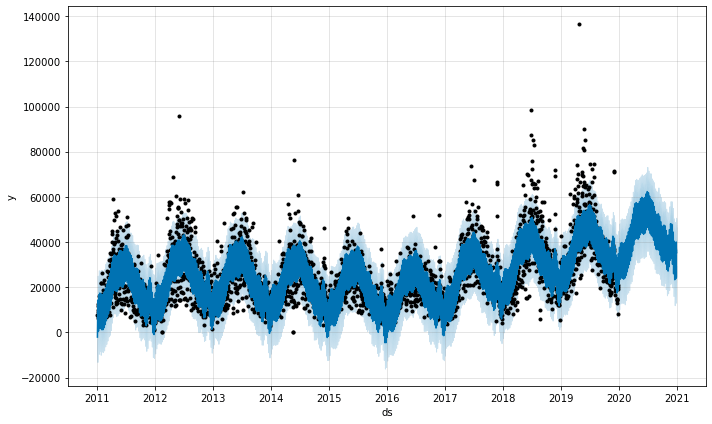
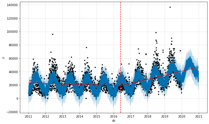
To examine the data we can use the model’s plot() method. This creates a really nice time series graph showing the four values from our dataframe above. The black dots represent the actual data, the dark blue line represents the model’s prediction, and the pale blue lines represent the upper and lower confidence interval.
As you can see, this retailer is experiencing a great upward trend in annual sales and experiences strong seasonality. The products it sells are linked to the weather, so those black dots that fall outside the usual range may well coincide with very good or very bad weather.
sales_forecast_plot = model.plot(forecast)
Examine underlying trends and seasonality
All ecommerce businesses experience trends and seasonality. Hopefully, the trend they experience is that their sales are rising over time, but the seasonality can be weekly (i.e. busy weekdays and quiet weekends) or yearly (i.e. busy in the summer and quiet in the winter).
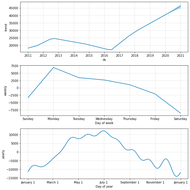
The plot_components() method uses Fourier transforms and dummy variables to extract the overall trend, and the weekly and yearly seasonality from the data set to show you all of the underlying patterns in your data. This gives us a clearer picture of what we observed above, minus the noise.
Firstly, we can see that sales for this retailer really picked up in summer 2016 and have been steadily growing ever since. The weekly seasonality component shows that Monday is the busiest day of the week, which drops towards the weekends, which tend to be pretty quiet by comparison. It’s also a very seasonal business, with sales peaking in the spring and early summer, and then declining as the weather gets cooler.
sales_forecast_components = model.plot_components(forecast)
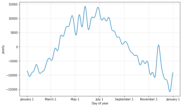
If you want to examine the seasonality in more granular detail, you can use the plot_yearly method and pass in the optional year_seasonality parameter when instantiating Prophet. Seasonal spikes are usually caused by natural demand increases (i.e. nice weather) and by holidays and key trading events, which can both occur at different times of the year. The Fourier series used here (see above) smooths this out so you see a more general trend, rather than the noise, which is what we’re seeing more of below. Could that December spike be Christmas shoppers, perhaps?
model_yearly = Prophet(yearly_seasonality=30, daily_seasonality=True).fit(df)
a = plot_yearly(model_yearly)
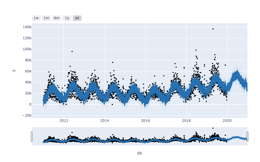
Exploring the forecast data interactively
The other real neat thing you can do is create interactive plots of your forecast using Plotly. These plots let you zoom in on the data to explore specific time periods so you can investigate why the model may not have predicted correctly, and also hover over the points to see what they represent.
plot_plotly(model, forecast)
Cross-validation
The simple model we’ve created above isn’t cross-validated. As you might imagine, cross-validation on time series data is really complicated, as you can’t simply slice up the dataset using train_test_split when the observations aren’t interchangeable. To explain how the Prophet model handles this, we first need to cover some special terminology: initial, cutoff, and horizon.
-
Initial: The initial represents the initial training period. On our data set, that initial period started in 2011 and ended in January 2020.
-
Cutoff (period): The cutoff starts at the end of the initial and finishes at the end of the horizon.
-
Horizon: The horizon represents the number of days to forecast after the end of the historic data, i.e. 30, 90, 180 or 365.
In order to cross-validate the data, Prophet measures forecasts on historical data using a method called Simulated Historical Forecasts (SHFs). Here the model creates cutoff points in history, refits the model on the initial data to that cutoff point and forecasts for a period for which it knows the actual results. It can then compare the forecast with the actual value to calculate model accuracy.
The cross_validation() method will handle this for you. You’ll just need to pass in the initial value (which is equal to the duration of your initial dataset minus the length of the horizon), the period (which is the number of days between cutoff dates), and the horizon, which is the number of days in the future to forecast.
initial_days = (df.ds.max() - df.ds.min()) / np.timedelta64(1, 'D')
period_days = initial_days - 365
period_days
2922.0
df_cv = cross_validation(model, initial='2922 days', period='180 days', horizon='365 days')
INFO:fbprophet:Making 1 forecasts with cutoffs between 2019-01-01 00:00:00 and 2019-01-01 00:00:00


HBox(children=(FloatProgress(value=0.0, max=1.0), HTML(value='')))
df_cv.head()
| ds | yhat | yhat_lower | yhat_upper | y | cutoff | |
|---|---|---|---|---|---|---|
| 0 | 2019-01-02 | 28038.281801 | 17971.989459 | 37393.649601 | 22926.5512 | 2019-01-01 |
| 1 | 2019-01-03 | 26827.267522 | 16493.746030 | 37243.240381 | 30695.3640 | 2019-01-01 |
| 2 | 2019-01-04 | 24040.108439 | 14612.662019 | 34148.993079 | 20672.2768 | 2019-01-01 |
| 3 | 2019-01-05 | 17756.237097 | 7642.141955 | 26936.184423 | 19642.1400 | 2019-01-01 |
| 4 | 2019-01-06 | 23262.631227 | 13276.440759 | 33611.007221 | 17414.9920 | 2019-01-01 |
cutoff = df_cv['cutoff'].unique()[0]
cutoff
numpy.datetime64('2019-01-01T00:00:00.000000000')
Measuring model performance
Now that we’ve cross-validated our model we can examine it’s performance. The performance_metrics() method computes a range of statistics on the cross validated data and returns the results in a Pandas dataframe. We get back the mean squared error (MSE), the root mean squared error (RMSE), the mean absolute error (MAE), the mean absolute percent error (MAPE), the median absolute percent error (MDAPE), and the coverage of the yhat_lower and yhat_upper estimates.
df_p = performance_metrics(df_cv)
df_p.head(10)
| horizon | mse | rmse | mae | mape | mdape | coverage | |
|---|---|---|---|---|---|---|---|
| 0 | 36 days | 2.808280e+07 | 5299.321127 | 4315.551126 | 0.194605 | 0.137002 | 0.944444 |
| 1 | 37 days | 2.743212e+07 | 5237.568042 | 4219.245369 | 0.190028 | 0.136523 | 0.944444 |
| 2 | 38 days | 2.823119e+07 | 5313.303286 | 4295.486436 | 0.195600 | 0.137002 | 0.944444 |
| 3 | 39 days | 2.863656e+07 | 5351.313635 | 4343.399081 | 0.200345 | 0.137002 | 0.944444 |
| 4 | 40 days | 2.889907e+07 | 5375.785223 | 4391.193894 | 0.202220 | 0.149592 | 0.944444 |
| 5 | 41 days | 2.876764e+07 | 5363.547306 | 4379.538083 | 0.197830 | 0.149592 | 0.944444 |
| 6 | 42 days | 3.671950e+07 | 6059.661878 | 4819.618695 | 0.226474 | 0.162616 | 0.916667 |
| 7 | 43 days | 3.599367e+07 | 5999.472464 | 4727.568623 | 0.222126 | 0.149592 | 0.916667 |
| 8 | 44 days | 3.846688e+07 | 6202.167382 | 4907.273537 | 0.231805 | 0.162616 | 0.888889 |
| 9 | 45 days | 3.725574e+07 | 6103.747911 | 4797.843043 | 0.226167 | 0.153729 | 0.888889 |
df_p.mean().to_frame()
| 0 | |
|---|---|
| horizon | 200 days 12:00:00 |
| mse | 1.31516e+08 |
| rmse | 10841.9 |
| mae | 8370.17 |
| mape | 0.243393 |
| mdape | 0.204946 |
| coverage | 0.683838 |
You can also examine these metrics in a range of visualisations. The general trend looks pretty good overall, but there’s a bit of fluctuation, which might be caused by weather conditions impacting sales, so they go outside the usual pattern.
fig = plot_cross_validation_metric(df_cv, metric='mse')
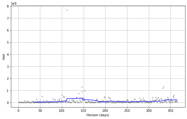
fig = plot_cross_validation_metric(df_cv, metric='rmse')
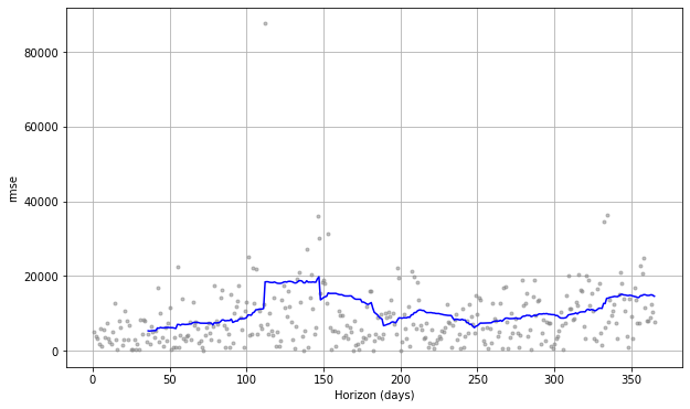
fig = plot_cross_validation_metric(df_cv, metric='mae')
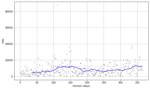
fig = plot_cross_validation_metric(df_cv, metric='mape')

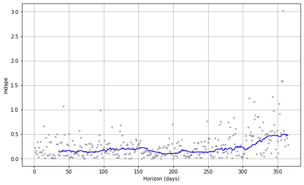
fig = plot_cross_validation_metric(df_cv, metric='mdape')
Understanding the impact of changepoints
The Prophet model uses features called “changepoints”. These are historic events that are associated with sudden changes in the trajectory of the forecast metric. So far, we’ve allowed Prophet to automatically identify the trend changepoints within our historic data. These growth-altering events might be positive things like sales, product launches, key trading calendar events, and negative things, like algorithm updates or site issues.
We’ll tune these important hyperparameters later, but before we do it’s worth having a play with them to see what they do. Sometimes, when there’s too much “flexibility” in the trend changes the model can overfit, while too little flexibility can cause underfitting. We can adjust these computationally when we undertake hyperparameter tuning, but it’s worth taking a look at what happens to the forecast when you change the changepoint setting manually to get an idea of what happens.
Prophet initially identifies loads of potential changepoints, and then reduces them to the main ones. To examine the changepoints on the default model, you can use the add_changepoints_to_plot() method. By default, they get placed only on the first 80% of the historic data, which is why they’re not present on the period in which the pandemic kicked off. Here are the changepoints on our default model again. By making adjustments to the changepoint settings we can change the fit of the model.
fig = model.plot(forecast)
a = add_changepoints_to_plot(fig.gca(), model, forecast)

Extracting changepoints
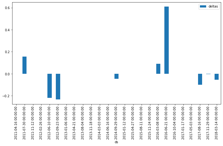
If you want to extract the changepoints detected and see what may have caused them, you can extract them from model.changepoints. The delta value is stored in the model.params. Once you’ve created a dataframe of changepoint deltas you can use Pandas to plot them.
points = pd.DataFrame(model.changepoints)
points['deltas'] = model.params['delta'].mean(0)
points.head()
| ds | deltas | |
|---|---|---|
| 105 | 2011-04-16 | 3.214285e-08 |
| 210 | 2011-07-30 | 1.556917e-01 |
| 315 | 2011-11-12 | 1.573965e-06 |
| 421 | 2012-02-26 | 3.990091e-10 |
| 526 | 2012-06-10 | -2.191237e-01 |
ax = points.plot.bar(x='ds', y='deltas', figsize=(12,6))
Default trend flexibility
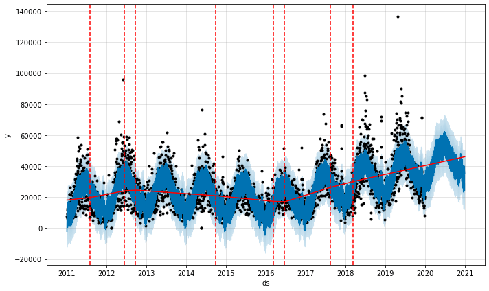
By default, the Prophet model uses a changepoint_prior_scale value of 0.05. If you plot the changepoints onto the forecast, you see that there’s a clear upward kick in the line as the model in the summer of 2016.
model = Prophet(changepoint_prior_scale=0.05)
forecast = model.fit(df).predict(future)

fig = model.plot(forecast)
a = add_changepoints_to_plot(fig.gca(), model, forecast)
INFO:fbprophet:Disabling daily seasonality. Run prophet with daily_seasonality=True to override this.
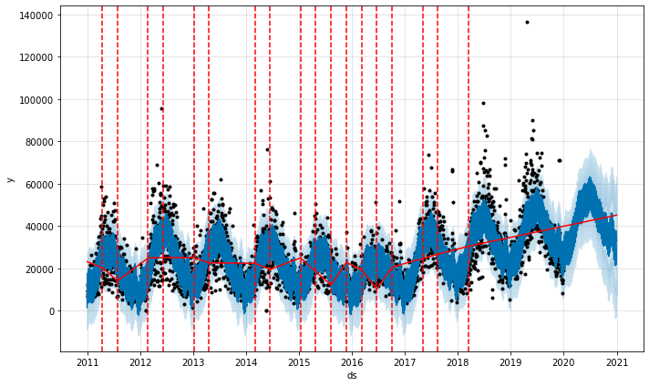
Increasing trend flexibility
To show what happens when you increase the trend flexibility, let’s refit the model and increase the changepoint_prior_scale from the default of 0.05 to 0.5. As you can see below, we get loads more changepoints identified and a much wider confidence interval for the future period. You can see from the graph that although the confidence interval is now much wider, it generally captures the trend better.
model = Prophet(changepoint_prior_scale=0.5)
forecast = model.fit(df).predict(future)

fig = model.plot(forecast)
a = add_changepoints_to_plot(fig.gca(), model, forecast)
INFO:fbprophet:Disabling daily seasonality. Run prophet with daily_seasonality=True to override this.
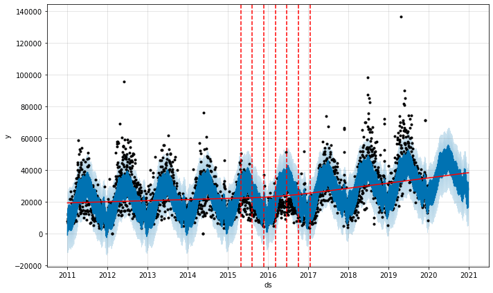
Decreasing trend flexibility
To show the opposite, we’ll pass in a lower value than the default (here 0.001 instead of 0.05). The changepoints are now concentrated around the period at which sales changed. This not only puts the actual forecast further outside the prediction, but also changes the overall slope of the forecast.
model = Prophet(changepoint_prior_scale=0.001)
forecast = model.fit(df).predict(future)

fig = model.plot(forecast)
a = add_changepoints_to_plot(fig.gca(), model, forecast)
INFO:fbprophet:Disabling daily seasonality. Run prophet with daily_seasonality=True to override this.
Manually defining changepoints
You can also specifically define the placement of changepoints. Here I’ve added a changepoint which coincides approximately with the change in the sales trend we observed in summer 2016. Obviously you’d normally include more than one in your list.
model = Prophet(changepoints=['2016-06-01'])
forecast = model.fit(df).predict(future)

fig = model.plot(forecast)
a = add_changepoints_to_plot(fig.gca(), model, forecast)
INFO:fbprophet:Disabling daily seasonality. Run prophet with daily_seasonality=True to override this.
Hyperparameter tuning
Now we have an idea of how change the changepoints affects the fit of the forecast we can tune them to find the right settings. As with other models, such as those in Scikit-Learn, you can use a Grid Search method to pass in a dictionary of model parameters and then test the model’s performance on each one through automated hyperparameter tuning.
As this process is a brute force approach which involves numerous iterations to find the best parameters, you may want to pass in the optional parallel='processes' argument to the cross_validation() method to speed things up by using more of your CPU threads. It can take a considerable amount of time to run, even on a powerful workstation.
Prophet allows you to tune many hyperparameters, the main ones are changepoint_prior_scale and seasonality_prior_scale, but holidays_prior_scale and seasonality_mode are also worth trying. Others tend to have less impact. Put each of the hyperparameters into a param_grid dictionary and include a range of values to test.
param_grid = {
    'changepoint_prior_scale': [0.001, 0.01, 0.1, 0.5, 0.75],
    'seasonality_prior_scale': [0.01, 0.1, 1.0, 10.0],
}
You can then use itertools to identify all of the unique parameter combinations and pass these into the model so it can try each one. After completion, it will store the RMSE value in the list so we can assess their performance.
all_params = [dict(zip(param_grid.keys(), v)) for v in itertools.product(*param_grid.values())]
rmses = []
Finally, we can loop through each set of parameters in the all_params list and fit the model to each one, run the cross validation and calculate and record the performance metrics.
for params in all_params:
    model = Prophet(**params, daily_seasonality=True).fit(df)

    df_cv = cross_validation(model, horizon='365 days')
    df_p = performance_metrics(df_cv, rolling_window=1)
    rmses.append(df_p['rmse'].values[0])

tuning_results = pd.DataFrame(all_params)
tuning_results['rmse'] = rmses
If you print out the tuning_results dataframe we populated above, you’ll see each pair of hyperparameters tried and the RMSE result obtained. Our lowest RMSE was when we fitted the model with changepoint_prior_scale set to 0.1 and seasonality_point_scale set to 0.01. You can extract the best parameters from all_params[np.argmin(rmses)].
best_params = all_params[np.argmin(rmses)]
best_params
{'changepoint_prior_scale': 0.1, 'seasonality_prior_scale': 0.01}
tuning_results.sort_values(by='rmse', ascending=True)
| changepoint_prior_scale | seasonality_prior_scale | rmse | |
|---|---|---|---|
| 8 | 0.100 | 0.01 | 9403.029293 |
| 11 | 0.100 | 10.00 | 9475.625811 |
| 10 | 0.100 | 1.00 | 9488.493826 |
| 9 | 0.100 | 0.10 | 9506.324298 |
| 17 | 0.750 | 0.10 | 9520.958539 |
| 19 | 0.750 | 10.00 | 9537.795263 |
| 13 | 0.500 | 0.10 | 9541.476890 |
| 15 | 0.500 | 10.00 | 9542.545616 |
| 14 | 0.500 | 1.00 | 9544.847108 |
| 18 | 0.750 | 1.00 | 9575.216643 |
| 4 | 0.010 | 0.01 | 9747.167005 |
| 5 | 0.010 | 0.10 | 9798.438722 |
| 6 | 0.010 | 1.00 | 9813.176997 |
| 7 | 0.010 | 10.00 | 9813.485803 |
| 0 | 0.001 | 0.01 | 11533.403949 |
| 2 | 0.001 | 1.00 | 11569.388314 |
| 1 | 0.001 | 0.10 | 11682.912308 |
| 3 | 0.001 | 10.00 | 11872.440834 |
| 12 | 0.500 | 0.01 | 12866.243262 |
| 16 | 0.750 | 0.01 | 14167.009321 |
By using plot_cross_validation_metric() we can plot some of the key metrics over time. The grey dots represent the absolute value for each prediction, while the blue line shows the RMSE, based on a rolling window of the dots. As you would imagine, the prediction for the near future is OK, but it gradually deteriorates over time.
fig = plot_cross_validation_metric(df_cv, metric='rmse')
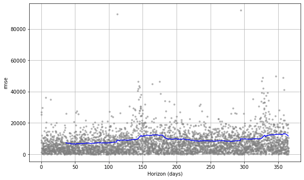
fig = plot_cross_validation_metric(df_cv, metric='mae')
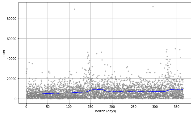
For this retailer, I think that the strong weather related impact might be making it much more challenging for the Prophet model to reliably forecast the result. If you work in a sector less influenced by weather, you should easily be able to achieve better and more consistent results than these. However, it’s possible to undertake further tuning for seasonality which we’ll tackle later by introducing some additional correlated regressors into our model.
df_p = performance_metrics(df_cv)
df_p.head()
| horizon | mse | rmse | mae | mdape | coverage | |
|---|---|---|---|---|---|---|
| 0 | 36 days 12:00:00 | 5.558822e+07 | 7455.751075 | 5513.094499 | 0.215407 | 0.830424 |
| 1 | 37 days 00:00:00 | 5.237557e+07 | 7237.097102 | 5412.819962 | 0.215407 | 0.833333 |
| 2 | 37 days 12:00:00 | 5.198136e+07 | 7209.810218 | 5380.386870 | 0.211243 | 0.835411 |
| 3 | 38 days 00:00:00 | 5.013534e+07 | 7080.631232 | 5348.938750 | 0.215372 | 0.837905 |
| 4 | 38 days 12:00:00 | 5.026598e+07 | 7089.850249 | 5358.017894 | 0.215372 | 0.837905 |
df_p.tail()
| horizon | mse | rmse | mae | mdape | coverage | |
|---|---|---|---|---|---|---|
| 653 | 363 days 00:00:00 | 1.552496e+08 | 12459.920397 | 9084.676190 | 0.307558 | 0.921031 |
| 654 | 363 days 12:00:00 | 1.498312e+08 | 12240.555534 | 8960.813596 | 0.302514 | 0.925187 |
| 655 | 364 days 00:00:00 | 1.456801e+08 | 12069.801558 | 8856.269949 | 0.303558 | 0.928928 |
| 656 | 364 days 12:00:00 | 1.408812e+08 | 11869.336686 | 8728.646466 | 0.300834 | 0.935162 |
| 657 | 365 days 00:00:00 | 1.358575e+08 | 11655.794274 | 8590.526883 | 0.294177 | 0.938903 |
Further reading
-
Samal, K.K.R., Babu, K.S., Das, S.K. and Acharaya, A., 2019, August. Time Series based Air Pollution Forecasting using SARIMA and Prophet Model. In Proceedings of the 2019 International Conference on Information Technology and Computer Communications (pp. 80-85).
-
Taylor, S.J. and Letham, B., 2018. Forecasting at scale. The American Statistician, 72(1), pp.37-45.
-
Usher, J. and Dondio, P., 2020, June. BREXIT Election: Forecasting a Conservative Party Victory through the Pound using ARIMA and Facebook’s Prophet. In Proceedings of the 10th International Conference on Web Intelligence, Mining and Semantics (pp. 123-128).
-
Yenidoğan, I., Çayir, A., Kozan, O., Dağ, T. and Arslan, Ç., 2018, September. Bitcoin forecasting using ARIMA and prophet. In 2018 3rd International Conference on Computer Science and Engineering (UBMK) (pp. 621-624). IEEE.
Matt Clarke, Saturday, March 06, 2021


Other posts you might like

How to tune a LightGBMClassifier model with Optuna
The LightGBM model is a gradient boosting framework that uses tree-based learning algorithms, much like the popular XGBoost model. LightGBM supports both classification and regression tasks, and is known for...

How to create a customer retention model with XGBoost
Although all business know the importance of retaining customers, few companies are actually able to measure customer retention accurately, and fewer still can predict which ones will churn or be...
