How to analyse search traffic using the Google Trends API
Google Trends data is now being used in a range of models. Here’s how you can access the data using PyTrends, an unofficial Google Trends API.
The things we search for online can reveal a remarkable amount about us, even when viewed in aggregate on an anonymous level. For many years, Google has made some of this search data available to browse via the Google Trends website, which allows you to plot the change in different search queries over time.
Google Trends data has long been used by those who work in ecommerce and marketing, as it gives you pointers on the terms people use and the changes in their popularity over time. This not only provides useful insight on the best keywords to use in content or the best products to promote, but the underlying data can also be used by data scientists within predictive models.
Using Google Trends data in models
The use of data from Google Trends in models isn’t a new thing and it’s been used in a number of different research fields, from finance to healthcare. Here’s a selection of some recent use cases from various papers:
Lyme disease: Seifter et al. (2010) used Google Trends data in epidemiological research monitoring the spread of Lyme disease, a potentially life threatening tick-borne infection. They were able to use data on searches for “lyme disease” to plot the areas in which Lyme disease was endemic and people were most at risk from infection.
Healthcare surveillance: Nuti et al. (2014) covered 70 medical studies that used Google Trends data for healthcare surveillance. They found four main trends: infectious diseases (27% of papers), mental health and substance abuse (24% of papers), non-communicable diseases (16% of papers), and general population behaviour (39% of papers).
Coronavirus: Strzelecki and Rizun (2020) examined searches for “coronavirus”, “sars”, and “mers”, and were able to identify the peaks in infection from search volumes, and identify the most affected regions. They found that Google Trends data forecasted the rise of new cases and suggested that national health services use it as an indicator of an incoming rise in patient numbers.
Nowcasting: Carrière‐Swallow and Labbé (2011) used Google Trends data for “nowcasting” in economic models. They showed that Google Trends data was useful because it wasn’t released with the “lag” seen in other economic metrics. Eichenauer et al. (2020) recently reported using this for examining daily sentiment.
Load the packages
In this project, we’ll look at how you can extract data from Google Trends to either gain insight or use it within models using the excellent PyTrends package. This works well, but as it’s unofficial, it comes with a risk that it may stop working if Google changes the way their data is accessible, so you need to be careful about using it in a production situation.
To get started, open a Jupyter notebook and install the PyTrends package using Pip if you don’t already have it installed. From the pytrends.request module import the TrendReq package and instantiate a new TrendReq() object. I’ve called mine pt for brevity. You can pass in various optional arguments when you instantiate TrendReq() including the timeout, the tz or timezone offset, a list of proxies if you’re blocked by Google, the number of retries and the host language or hl.
!pip install pytrends
import pandas as pd
from pytrends.request import TrendReq
import matplotlib.pyplot as plt

%matplotlib inline
plt.rcParams["figure.figsize"] = [16, 6]
pt = TrendReq()
Trending searches
The trending_searches() function returns a dataframe containing the current most popular searches being entered on Google. By default, if you pass in no arguments trending_searches() returns the top global searches.
df = pt.trending_searches()
df.head(5)
| 0 | |
|---|---|
| 0 | Earthquake |
| 1 | Iowa Governor Kim Reynolds |
| 2 | Chicago Bears |
| 3 | Moderna stock |
| 4 | Chris Paul |
If you want to examine the specific trending searches for a region, you can pass in a value with the pn argument. This takes the name of the country in lower case letters with spaces replaced by underscores, i.e. united_kingdom, or united_states.
df = pt.trending_searches(pn='united_kingdom')
df.head(5)
| 0 | |
|---|---|
| 0 | Scooter Braun |
| 1 | Scotland lockdown |
| 2 | Ryan Reynolds |
| 3 | Moderna |
| 4 | Boris Johnson |
Interest over time
To examine and chart the interest of specific search queries over time you can use the interest_over_time() function. To use this you initially need to build a PyTrends payload, which takes a list of search terms. It will return the search volume for each time period and each term in a Pandas dataframe.
pt.build_payload(['testicular cancer', 'movember'])
df = pt.interest_over_time()
df.head()
| testicular cancer | movember | isPartial | |
|---|---|---|---|
| date | |||
| 2015-11-22 | 12 | 48 | False |
| 2015-11-29 | 12 | 30 | False |
| 2015-12-06 | 11 | 6 | False |
| 2015-12-13 | 11 | 3 | False |
| 2015-12-20 | 10 | 5 | False |
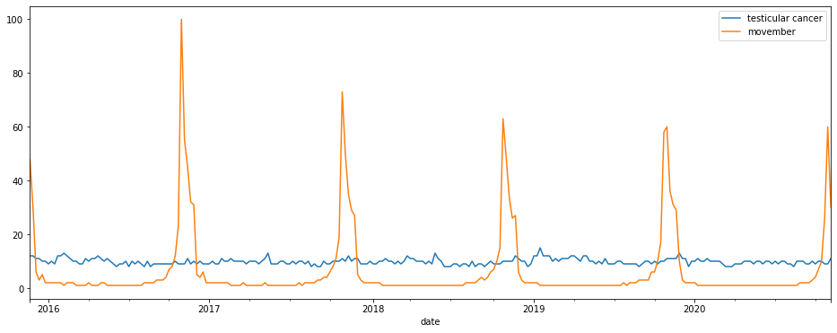
To plot the search terms over time you can use the built-in Pandas plot() function. This will automatically take the date-indexed dataframe and displaying each search term with a different colour line. Let’s examine the relationship between “Movember” and “testicular cancer” to see how it’s increased awareness.
df.plot()
YouTube trends
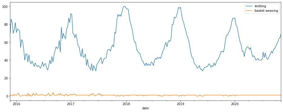
You can also run Google Trends searches on other Google properties, besides the default Google search. Let’s take a look at YouTube searches for “knitting” and “basket weaving” to see how demand differs and whether there’s any seasonality.
pt.build_payload(['knitting', 'basket weaving'], gprop='youtube')
df = pt.interest_over_time()
df.plot()
Google News trends
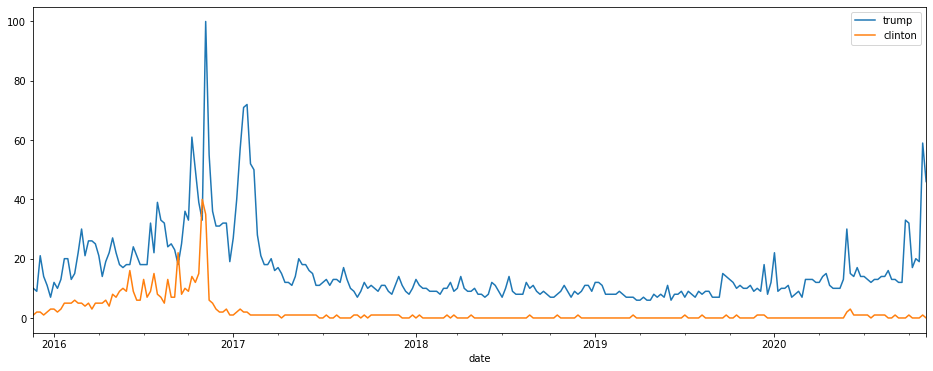
Similarly, you can also restrict your searches to examine the Google News property. Here’s a plot of “trump” versus “clinton”.
pt.build_payload(['trump', 'clinton'], gprop='news')
df = pt.interest_over_time()
df.plot()
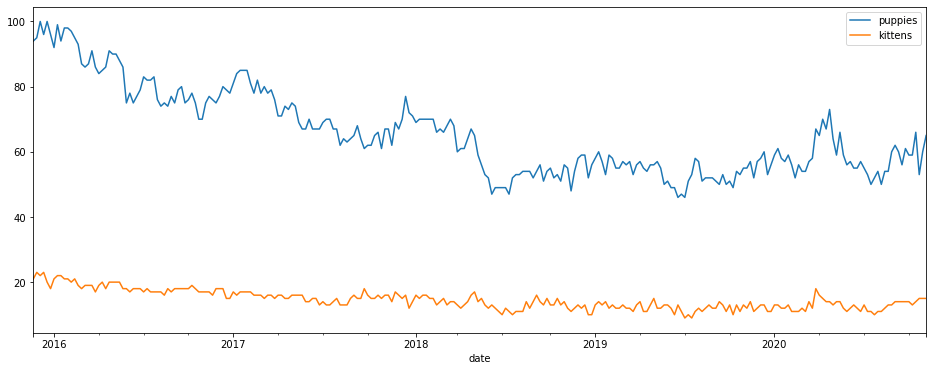
Google Images trends
Search trends on Google Images can be undertaken by passing in the images value to the gprop parameter. Here’s “puppies” versus “kittens”. Looks like puppies are not as popular as they once were…
pt.build_payload(['puppies', 'kittens'], gprop='images')
df = pt.interest_over_time()
df.plot()
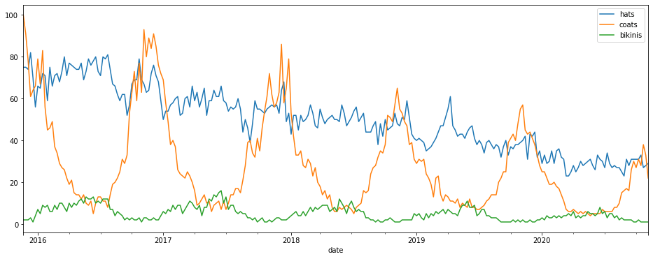
Google Shopping trends
For retailers, the Google Shopping trends data is perhaps of most interest. This is accessed via the froogle argument in gprop as Froogle used to be the old name for Google Shopping. Here’s the seasonality and changes in search volumes on Google Shopping for a few items of clothing and millinery.
pt.build_payload(['hats', 'coats', 'bikinis'], gprop='froogle')
df = pt.interest_over_time()
df.plot()
Interest by region
You can also examine the specific interest in a search query across different regions. This uses the interest_by_region() function which uses a query payload from build_payload(). This function accepts various arguments that allow you to control the output.
query = 'electric scooters'
pt.build_payload(kw_list=[query])
df = pt.interest_by_region(resolution='COUNTRY', inc_low_vol=True, inc_geo_code=True)
scooters = df.sort_values(by=query, ascending=False).head(10)
scooters.reset_index()
| geoName | geoCode | electric scooters | |
|---|---|---|---|
| 0 | Ireland | IE | 100 |
| 1 | United Kingdom | GB | 97 |
| 2 | New Zealand | NZ | 87 |
| 3 | Australia | AU | 66 |
| 4 | Malta | MT | 63 |
| 5 | United States | US | 52 |
| 6 | Canada | CA | 43 |
| 7 | St. Helena | SH | 36 |
| 8 | Cyprus | CY | 31 |
| 9 | Singapore | SG | 30 |
Top charts
To get a historic view of what we were searching for in years gone by you can use the top_charts() function. In 2002, it seems we were all into “David Beckham” and “Anna Kournikova”.
pt.top_charts('2002', hl='en-GB', tz=300, geo='GLOBAL')
| title | exploreQuery | |
|---|---|---|
| 0 | David Beckham | |
| 1 | Anna Kournikova | |
| 2 | Ronaldo | |
| 3 | Kobe Bryant | |
| 4 | Zinedine Zidane | |
| 5 | Vince Carter | |
| 6 | Allen Iverson | |
| 7 | Serena Williams | |
| 8 | Tiger Woods | |
| 9 | Venus Williams |
Suggestions
While not technically part of Google Trends, the PyTrends package also gives you access to both keyword suggestions (and disambiguation data) and related queries. The latter can be very useful in SEO, as it tells you the approximate level of search interest in phrases so you can incorporate the terms into your copywriting.
Disambiguation
suggestions = pt.suggestions(keyword='Pandas')
df = pd.DataFrame(suggestions).drop(columns='mid')
df.head()
| title | type | |
|---|---|---|
| 0 | pandas | Software |
| 1 | PANDAS | Disorder |
| 2 | Pandas | Animal |
| 3 | Red pandas | Animal |
| 4 | Giant Pandas | Animal |
Related queries
pt.build_payload(['sklearn', 'pandas', 'python', 'data science', 'machine learning'], cat=5)
related = pt.related_queries()
related['data science']['top'].head()
| query | value | |
|---|---|---|
| 0 | python | 100 |
| 1 | data science python | 100 |
| 2 | computer science | 68 |
| 3 | analytics | 44 |
| 4 | bootcamp data science | 43 |
related['data science']['rising'].head()
| query | value | |
|---|---|---|
| 0 | jupyter notebook | 70050 |
| 1 | laptops for data science | 52650 |
| 2 | upgrad data science | 49200 |
| 3 | upgrad | 48100 |
| 4 | python libraries for data science | 43450 |
Further reading
- Carrière‐Swallow, Y. and Labbé, F., 2013. Nowcasting with Google Trends in an emerging market. Journal of Forecasting, 32(4), pp.289-298.
- Eichenauer, V., Indergand, R., Martínez, I.Z. and Sax, C., 2020. Constructing daily economic sentiment indices based on Google trends. KOF Working Papers, 484.
- Kurian, S.J., Alvi, M.A., Ting, H.H., Storlie, C., Wilson, P.M., Shah, N.D., Liu, H. and Bydon, M., 2020, August. Correlations Between COVID-19 Cases and Google Trends Data in the United States: A State-by-State Analysis. In Mayo Clinic Proceedings. Elsevier.
- Nuti, S.V., Wayda, B., Ranasinghe, I., Wang, S., Dreyer, R.P., Chen, S.I. and Murugiah, K., 2014. The use of google trends in health care research: a systematic review. PloS one, 9(10), p.e109583.
- Pelat, C., Turbelin, C., Bar-Hen, A., Flahault, A. and Valleron, A.J., 2009. More diseases tracked by using Google Trends. Emerging infectious diseases, 15(8), p.1327.
- Seifter, A., Schwarzwalder, A., Geis, K. and Aucott, J., 2010. The utility of “Google Trends” for epidemiological research: Lyme disease as an example. Geospatial health, pp.135-137.
- Strzelecki, A. and Rizun, M., 2020. Infodemiological study using google trends on coronavirus epidemic in Wuhan, China.
Matt Clarke, Saturday, March 06, 2021


Other posts you might like

How to use the Pandas truncate() function
Have you ever needed to chop the top or bottom off a Pandas dataframe, or extract a specific section from the middle? If so, there’s a Pandas function called truncate()...

How to use Spacy for noun phrase extraction
Noun phrase extraction is a Natural Language Processing technique that can be used to identify and extract noun phrases from text. Noun phrases are phrases that function grammatically as nouns...
