How to calculate Spearman's rank correlation coefficient in Pandas
Learn to calculate the Spearman's rank correlation coefficient, or Spearman's rho, using the Pandas corr() statistical method.

Spearman’s rank correlation coefficient, sometimes called Spearman’s rho, is a nonparametric statistic used to measure rank correlation, or the statistical dependence between the rankings of two variables. It explains how well a statistical relationship between two variables can be explained using a monotonic function.
While Pearson’s correlation coefficient is used to measure the relationship between pairs of variables with a linear relationship, Spearman’s rank correlation coefficient assesses monotonic relationships, whether they’re linear or not. It’s a non-parametric measure of correlation, meaning that it doesn’t assume that the data is normally distributed.
As the name suggests, it’s a measure of rank correlation, meaning that it’s based on the ranks of the data rather than the data itself. This is important because it means that it’s not affected by outliers, which can skew Pearson’s correlation coefficient. Spearman’s rank correlation is equal to the Pearson correlation coefficient of the ranks of the data and, like Pearson’s correlation coefficient, it ranges from -1 to 1.
When should you use Spearman’s rank correlation coefficient?
Spearman’s rank correlation coefficient is a nonparametric measure of the monotonicity of the relationship between two datasets. Unlike the Pearson correlation, the Spearman correlation does not assume that both datasets are normally distributed.
It is often used as an alternative to the Pearson correlation in the presence of outliers and can be useful for both continuous and ordinal variables. It assumes that the data must at least be ordinal and the scores on one variable need to be related monotonically to the other variable in the pairwise comparison.
It’s typically used on ordinal or continuous variables, but it can also be used on nominal variables. It’s often used in place of Pearson’s correlation coefficient when the data is not normally distributed.
Spearman’s rank correlation coefficient using corr()
The Pandas corr() function can be used to compute pairwise correlation coefficients, including Spearman’s rho, on Pandas dataframe values, and can either calculate them as individual pairs (i.e. top speed and price), or as pairs across an entire dataframe.
By default, the corr() function calculates the more commonly used Pearson’s correlation coefficient, but it can be easily modified to return the Spearman’s rank correlation coefficient, or Spearman’s rho, by passing in the optional argument method='spearman'. Here’s a quick summary of the parameters you can pass to the Pandas corr() function.
| Parameter | Description |
|---|---|
method |
The method parameter defines which of the three correlation coefficient methods to use. The default is pearson, which is the Pearson product-moment correlation coefficient. The other two methods are kendall, for the Kendall Tau correlation coefficient, and spearman for the Spearman rank correlation coefficient. |
min_periods |
The min_periods parameter defines the minimum number of observations required to calculate the correlation coefficient. If there are fewer than min_periods observations, the correlation coefficient will be set to NaN. This currently only works when the method parameter is set to pearson or spearman. |
numeric_only |
The numeric_only parameter was new in Pandas 1.5.0, so it won't work on earlier releases of Pandas. This parameter defines whether to only calculate the correlation coefficient on numeric columns. If set to True, only numeric columns will be used to calculate the correlation coefficient. If set to False, all columns will be used to calculate the correlation coefficient. The default is True. In a future release, the value of numeric_only will change to False, so if you don't set it you'll currently get this warning:
"FutureWarning: The default value of numeric_only in DataFrame.corr is deprecated. In a future version, it will default to False. Select only valid columns or specify the value of numeric_only to silence this warning." Passing numeric_only=True will fix it.
|
Interpreting Spearman’s rho
When you use the optional method='spearman' option, the corr() function will return the Spearman’s rank correlation coefficient for each pair of columns in the dataframe. The correlation coefficient returned, will be a value between -1 and +1. Here’s how you can interpret what these coefficients mean:
| Spearman's rho value | Strength of relationship |
|---|---|
| -1 | Perfect negative linear relationship |
| -0.7 | Strong negative linear relationship |
| -0.5 | Moderate negative linear relationship |
| -0.3 | Weak negative linear relationship |
| 0 | No linear relationship |
| 0.3 | Weak positive linear relationship |
| 0.5 | Moderate positive linear relationship |
| 0.7 | Strong positive linear relationship |
| 1 | Perfect positive linear relationship |
Load the packages
To work through some simple examples showing how to compute Spearman’s rank correlation in Python we’ll be using Pandas. To get started, import Pandas in a Jupyter notebook. We’ll also use the Matplotlib and Seaborn data visualisation libraries to visualise the Spearman rank correlation, and we’ll use Scipy Stats to test the statistical significance.
import pandas as pd
import matplotlib.pyplot as plt
import seaborn as sns
from scipy.stats import spearmanr
Import a dataset
Next, import a dataset into Pandas that contains data with linear relationships. I’m using a house price dataset.
df = pd.read_csv('https://raw.githubusercontent.com/flyandlure/datasets/master/housing.csv')
df.head().T
| 0 | 1 | 2 | 3 | 4 | |
|---|---|---|---|---|---|
| longitude | -122.23 | -122.22 | -122.24 | -122.25 | -122.25 |
| latitude | 37.88 | 37.86 | 37.85 | 37.85 | 37.85 |
| housing_median_age | 41.0 | 21.0 | 52.0 | 52.0 | 52.0 |
| total_rooms | 880.0 | 7099.0 | 1467.0 | 1274.0 | 1627.0 |
| total_bedrooms | 129.0 | 1106.0 | 190.0 | 235.0 | 280.0 |
| population | 322.0 | 2401.0 | 496.0 | 558.0 | 565.0 |
| households | 126.0 | 1138.0 | 177.0 | 219.0 | 259.0 |
| median_income | 8.3252 | 8.3014 | 7.2574 | 5.6431 | 3.8462 |
| median_house_value | 452600.0 | 358500.0 | 352100.0 | 341300.0 | 342200.0 |
| ocean_proximity | NEAR BAY | NEAR BAY | NEAR BAY | NEAR BAY | NEAR BAY |
Calculate the Spearman’s rank correlation for a pair of columns
To calculate Spearman’s rank correlation on a single pair of Pandas dataframe columns we’ll use the Pandas corr() function with the method parameter set to spearman. To use the function we run df['median_income'].corr(df['median_house_value'], method='spearman'), where the first column is the column we want to compare to the second column.
df['median_income'].corr(df['median_house_value'], method='spearman')
0.6767781095942506
Calculate the Spearman’s rank correlation for all columns in the dataframe
To calculate the Spearman’s rank correlation for all columns in a Pandas dataframe we can use the corr() method with the method parameter set to spearman, but we’ll assign this to df rather than a single column, and we won’t pass in another column to compare against.
At present, you’ll need to set numeric_only=True to avoid getting a FutureWarning about the default value changing to False in a future version of Pandas.
df.corr(numeric_only=True, method='spearman')
| longitude | latitude | housing_median_age | total_rooms | total_bedrooms | population | households | median_income | median_house_value | |
|---|---|---|---|---|---|---|---|---|---|
| longitude | 1.000000 | -0.879203 | -0.150752 | 0.040120 | 0.063879 | 0.123527 | 0.060020 | -0.009928 | -0.069667 |
| latitude | -0.879203 | 1.000000 | 0.032440 | -0.018435 | -0.056636 | -0.123626 | -0.074299 | -0.088029 | -0.165739 |
| housing_median_age | -0.150752 | 0.032440 | 1.000000 | -0.357162 | -0.306544 | -0.283879 | -0.281989 | -0.147308 | 0.074855 |
| total_rooms | 0.040120 | -0.018435 | -0.357162 | 1.000000 | 0.915021 | 0.816185 | 0.906734 | 0.271321 | 0.205952 |
| total_bedrooms | 0.063879 | -0.056636 | -0.306544 | 0.915021 | 1.000000 | 0.870937 | 0.975627 | -0.006196 | 0.086259 |
| population | 0.123527 | -0.123626 | -0.283879 | 0.816185 | 0.870937 | 1.000000 | 0.903872 | 0.006268 | 0.003839 |
| households | 0.060020 | -0.074299 | -0.281989 | 0.906734 | 0.975627 | 0.903872 | 1.000000 | 0.030305 | 0.112737 |
| median_income | -0.009928 | -0.088029 | -0.147308 | 0.271321 | -0.006196 | 0.006268 | 0.030305 | 1.000000 | 0.676778 |
| median_house_value | -0.069667 | -0.165739 | 0.074855 | 0.205952 | 0.086259 | 0.003839 | 0.112737 | 0.676778 | 1.000000 |
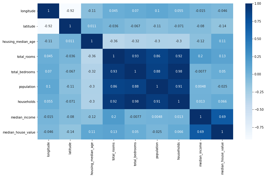
Visualise Spearman’s rank correlation coefficients with a heatmap
By using Seaborn, we can visualise the Spearman’s rank correlation coefficients using a heatmap visualisation of correlation coefficients. This can be an effective way to quickly understand relationships between data, as you can simply lookup those values where the correlation is strongly negative or strongly positive.
plt.figure(figsize=(14,8))
sns.heatmap(df.corr(numeric_only=True), annot=True, cmap='Blues')
<AxesSubplot:>
Visualising correlations between pairs of columns
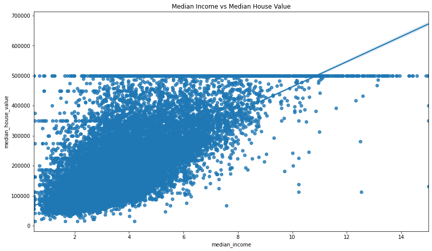
You can also use Seaborn to examine the relationship between a specific pair of variables that appear to have a strong correlation. The Seaborn regplot() function is great for this.
plt.figure(figsize=(14,8))
sns.regplot(x='median_income', y='median_house_value', data=df)
plt.title('Median Income vs Median House Value')
Text(0.5, 1.0, 'Median Income vs Median House Value')
Calculate the statistical significance of the correlation coefficient
Finally, you can measure the statistical significance of Spearman’s rho using Scipy Stats. Scipy Stats calculates both the correlation coefficient of a pair of variables as well as their statistical significance, but it’s clunkier to use than Pandas, so tends to be used mostly to validate whether a correlation is significant or not.
To use it, you simply call spearmanr() and pass in the two Pandas columns you want to compare. By comparing the median_income and median_house_value columns we get back a moderately strong correlation and a statistically significant p value.
spearmanr(df['median_income'], df['median_house_value'])
SpearmanrResult(correlation=0.6767781095942506, pvalue=0.0)
By contrast, if you use Scipy to calculate the Spearman’s rank correlation coefficient and p value of the housing_median_age and median_house_value columns you get back a higher p value, indicating that the result is not statistically significant.
spearmanr(df['housing_median_age'], df['median_house_value'])
SpearmanrResult(correlation=0.07485485302251019, pvalue=4.844329494934632e-27)
Matt Clarke, Friday, December 02, 2022


Other posts you might like

How to use the Pandas truncate() function
Have you ever needed to chop the top or bottom off a Pandas dataframe, or extract a specific section from the middle? If so, there’s a Pandas function called truncate()...

How to use Spacy for noun phrase extraction
Noun phrase extraction is a Natural Language Processing technique that can be used to identify and extract noun phrases from text. Noun phrases are phrases that function grammatically as nouns...
