How to calculate Pearson correlation coefficient in Pandas
Learn to use the Pandas corr() statistical method to compute the Pearson correlation coefficient (PCC), Pearson's r, or the Pearson Product Moment Correlation (PPMCC) in Pandas.

The Pearson correlation coefficient, or PCC, is the standard statistical method for computing pairwise or bivariate correlation in Pandas. It’s so commonly used in statistics, that it is often referred to simply as “the correlation coefficient.” Pearson correlation coefficient is exactly the same thing as Pearson’s r, and the Pearson product moment correlation coefficient (PPMCC), it just has several names.
As with other correlation coefficients, Pearson correlation is used to compute the strength of linear correlation between two variables in a dataset. It’s basically the ratio between the covariance of the variables and the product of their standard deviations, and gives a normalised measure of covariance that returns a value between 1 and -1. A value of 1 indicates a perfect positive linear relationship, a value of -1 indicates a perfect negative linear relationship, and a value of 0 indicates no linear relationship.
By interpreting the result of the Pearson correlation coefficient you can tell whether one variable is associated with a change in the other. For example, the price of new cars might be positively correlated with top speed, since most very expensive new cars are supercars or hypercars.
In this tutorial, I’ll explain Pearson correlation and show how you can use it to spot correlations between variables in your dataset using the Pandas corr() function.
Pearson correlation coefficient using corr()
The Pearson correlation coefficient can be easily calculated in Pandas using corr(). The corr() function is used to compute pairwise correlation coefficients on Pandas dataframe values, and can either calculate them as individual pairs (i.e. top speed and price), or as pairs across an entire dataframe.
Since Pearson correlation coefficient is so widely used by statisticians and data scientists, the corr() function is pre-configured with default values to return the Pearson correlation coefficient. However, you can change this to use the similar Spearman rank correlation (or Spearman’s r), or the Kendall Tau correlation coefficient, if you think they better suit your data.
The corr() function takes three arguments, all of which are optional. Here’s a quick summary of what they do.
| Parameter | Description |
|---|---|
method |
The method parameter defines which of the three correlation coefficient methods to use. The default is pearson, which is the Pearson product-moment correlation coefficient. The other two methods are kendall, for the Kendall Tau correlation coefficient, and spearman for the Spearman's rank correlation coefficient. |
min_periods |
The min_periods parameter defines the minimum number of observations required to calculate the correlation coefficient. If there are fewer than min_periods observations, the correlation coefficient will be set to NaN. This currently only works when the method parameter is set to pearson or spearman. |
numeric_only |
The numeric_only parameter was new in Pandas 1.5.0, so it won't work on earlier releases of Pandas. This parameter defines whether to only calculate the correlation coefficient on numeric columns. If set to True, only numeric columns will be used to calculate the correlation coefficient. If set to False, all columns will be used to calculate the correlation coefficient. The default is True. In a future release, the value of numeric_only will change to False, so if you don't set it you'll currently get this warning:
"FutureWarning: The default value of numeric_only in DataFrame.corr is deprecated. In a future version, it will default to False. Select only valid columns or specify the value of numeric_only to silence this warning." Passing numeric_only=True will fix it.
|
Interpreting Pearson’s correlation coefficient
When using corr(method='pearson'), or just corr(), since method='pearson' is the default, the resulting correlation matrix will have a value for every pair of columns in the original DataFrame.
The value will be a number between -1 and 1, where 1 is a perfect positive linear relationship, 0 is no linear relationship, and -1 is a perfect negative linear relationship. Different authors use slightly different interpretations of the coefficients, but they’re generally very similar to the ones below.
| Pearson's r value | Strength of relationship |
|---|---|
| 0 | No linear relationship |
| 0.1 to 0.3 | Weak linear relationship |
| 0.3 to 0.5 | Moderate linear relationship |
| 0.5 to 0.7 | Strong linear relationship |
| 0.7 to 1 | Very strong linear relationship |
| -0.1 to -0.3 | Weak negative linear relationship |
| -0.3 to -0.5 | Moderate negative linear relationship |
| -0.5 to -0.7 | Strong negative linear relationship |
| -0.7 to -1 | Very strong negative linear relationship |
Load the packages
To get started, open a new Jupyter notebook and import the Pandas library. You only need this to calculate correlation coefficients in Pandas, but to cover some more advanced topics we’ll also import the Matplotlib and Seaborn data visualisation packages, and the Scipy statistical analysis package.
import pandas as pd
import matplotlib.pyplot as plt
import seaborn as sns
from scipy.stats import pearsonr
Import a dataset
Then, either create a dummy dataset of data with linear relationships between the variables, or import a dataset into Pandas from a CSV file. I’m using a house price dataset, as this contains several correlated variables.
df = pd.read_csv('https://raw.githubusercontent.com/flyandlure/datasets/master/housing.csv')
df.head().T
| 0 | 1 | 2 | 3 | 4 | |
|---|---|---|---|---|---|
| longitude | -122.23 | -122.22 | -122.24 | -122.25 | -122.25 |
| latitude | 37.88 | 37.86 | 37.85 | 37.85 | 37.85 |
| housing_median_age | 41.0 | 21.0 | 52.0 | 52.0 | 52.0 |
| total_rooms | 880.0 | 7099.0 | 1467.0 | 1274.0 | 1627.0 |
| total_bedrooms | 129.0 | 1106.0 | 190.0 | 235.0 | 280.0 |
| population | 322.0 | 2401.0 | 496.0 | 558.0 | 565.0 |
| households | 126.0 | 1138.0 | 177.0 | 219.0 | 259.0 |
| median_income | 8.3252 | 8.3014 | 7.2574 | 5.6431 | 3.8462 |
| median_house_value | 452600.0 | 358500.0 | 352100.0 | 341300.0 | 342200.0 |
| ocean_proximity | NEAR BAY | NEAR BAY | NEAR BAY | NEAR BAY | NEAR BAY |
Calculate the Pearson correlation for a pair of columns
To calculate the Pearson correlation for a pair of columns, you can append the .corr() method to the first column and pass the second column as an argument. If we do this for the median_income and median_house_value columns we get back a PCC or r of 0.6880, which according to our interpretation in the lookup table denotes a strong linear correlation. That means, samples with a higher median_income generally had a higher median_house_value.
df['median_income'].corr(df['median_house_value'])
0.688075207958548
Calculate the Pearson correlation for all columns in the dataframe
To calculate the Pearson correlation coefficient for every pair of values in the dataframe, you can simply append the corr() method to the end of the dataframe object. The resulting dataframe, or matrix, will have the correlation coefficient for every pair of columns in the dataframe. To avoid getting a FutureWarning, you’ll want to set numeric_only=True in the corr() method.
df.corr(numeric_only=True)
| longitude | latitude | housing_median_age | total_rooms | total_bedrooms | population | households | median_income | median_house_value | |
|---|---|---|---|---|---|---|---|---|---|
| longitude | 1.000000 | -0.924664 | -0.108197 | 0.044568 | 0.069608 | 0.099773 | 0.055310 | -0.015176 | -0.045967 |
| latitude | -0.924664 | 1.000000 | 0.011173 | -0.036100 | -0.066983 | -0.108785 | -0.071035 | -0.079809 | -0.144160 |
| housing_median_age | -0.108197 | 0.011173 | 1.000000 | -0.361262 | -0.320451 | -0.296244 | -0.302916 | -0.119034 | 0.105623 |
| total_rooms | 0.044568 | -0.036100 | -0.361262 | 1.000000 | 0.930380 | 0.857126 | 0.918484 | 0.198050 | 0.134153 |
| total_bedrooms | 0.069608 | -0.066983 | -0.320451 | 0.930380 | 1.000000 | 0.877747 | 0.979728 | -0.007723 | 0.049686 |
| population | 0.099773 | -0.108785 | -0.296244 | 0.857126 | 0.877747 | 1.000000 | 0.907222 | 0.004834 | -0.024650 |
| households | 0.055310 | -0.071035 | -0.302916 | 0.918484 | 0.979728 | 0.907222 | 1.000000 | 0.013033 | 0.065843 |
| median_income | -0.015176 | -0.079809 | -0.119034 | 0.198050 | -0.007723 | 0.004834 | 0.013033 | 1.000000 | 0.688075 |
| median_house_value | -0.045967 | -0.144160 | 0.105623 | 0.134153 | 0.049686 | -0.024650 | 0.065843 | 0.688075 | 1.000000 |
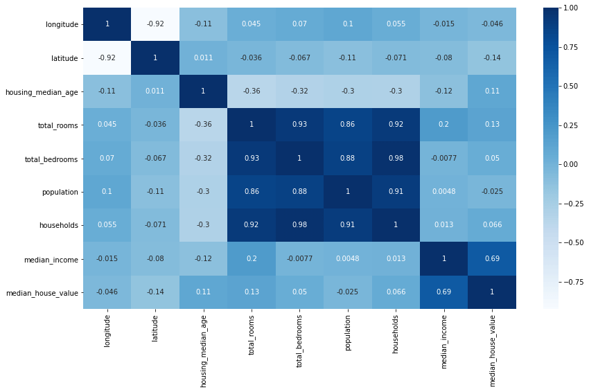
Visualise the correlation coefficients with a heatmap
When examining a dataset it’s often easier to visualise the correlations using Seaborn, or a similar data visualisation library. Visualising the correlations via a heatmap is my preferred technique and is easily done by using just a Seaborn function and a Matplotlib function to adjust the figure size.
plt.figure(figsize=(14,8))
sns.heatmap(df.corr(numeric_only=True), annot=True, cmap='Blues')
<AxesSubplot:>
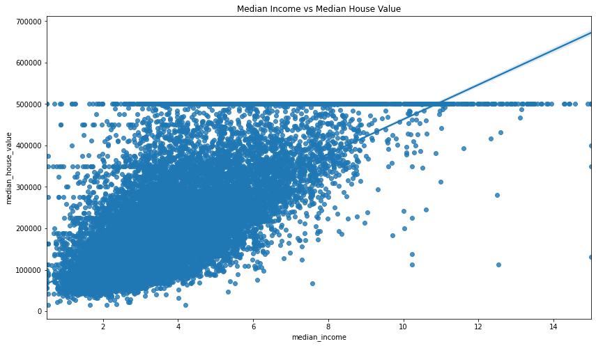
Visualising correlations between pairs of columns
There are various ways to visualise correlations between pairs of variables. A quick way to view the correlations of a single pair is to use the Seaborn regplot() function. This takes three arguments comprising the x and y columns you want to plot, and the data from the dataframe.
plt.figure(figsize=(14,8))
sns.regplot(x='median_income', y='median_house_value', data=df)
plt.title('Median Income vs Median House Value')
Text(0.5, 1.0, 'Median Income vs Median House Value')
Calculate the statistical significance of the correlation coefficient
To determine whether the correlation coefficient is statistically significant or not you can use the pearsonr() method from scipy.stats. This returns does much the same as the Pandas corr() function, in that it also returns the correlation coefficient, but crucially, it provides the p-value that Pandas does not.
The p-value is the probability that the correlation coefficient is not statistically significant. If the p-value is less than 0.05 then the correlation coefficient is statistically significant. We get a very low p value, so the correlation coefficient is statistically significant.
pearsonr(df['median_income'], df['median_house_value'])
(0.6880752079585477, 0.0)
By contrast, if you use Scipy to calculate the Pearson correlation coefficient and p value of the housing_median_age and median_house_value columns you get back a higher p value, indicating that the result is not statistically significant.
pearsonr(df['housing_median_age'], df['median_house_value'])
(0.10562341249320992, 2.7618606761502365e-52)
Matt Clarke, Sunday, November 20, 2022


Other posts you might like

How to use the Pandas truncate() function
Have you ever needed to chop the top or bottom off a Pandas dataframe, or extract a specific section from the middle? If so, there’s a Pandas function called truncate()...

How to use Spacy for noun phrase extraction
Noun phrase extraction is a Natural Language Processing technique that can be used to identify and extract noun phrases from text. Noun phrases are phrases that function grammatically as nouns...
