How to use model selection and hyperparameter tuning
Model selection and hyperparameter tuning can greatly improve model performance. Learn how to use these techniques through XGBRegressor hyperparameter tuning.

There are many techniques you can apply to improve the performance of your machine learning models, but two of the most powerful are model selection and hyperparameter tuning. As models perform differently on different datasets, it’s useful to test several models, rather than simply accept the first one through a computational approach called model selection.
Similarly, when you train a model using its default parameters they might give OK results, but you can usually gain a little extra performance by applying hyperparameter tuning to find the optimum combination for the best score. To show how the model selection and hyperparameter tuning steps work, we’ll see what sort of improvement we can get on a linear regression model.
Load the packages
First, fire up a Jupyter notebook and load up the below packages. These include Pandas and Numpy for data manipulation, Seaborn and Matplotlib for plotting, plus a range of Scikit-Learn packages for creating and validating regression models.
import time
import pandas as pd
import numpy as np
import seaborn as sns
import matplotlib.pyplot as plt
from sklearn.preprocessing import StandardScaler
from sklearn.model_selection import train_test_split
from sklearn.metrics import mean_squared_error
from sklearn.model_selection import RepeatedStratifiedKFold
from sklearn.model_selection import GridSearchCV, RandomizedSearchCV
from sklearn.model_selection import cross_val_score
from xgboost import XGBRegressor
from sklearn.tree import DecisionTreeRegressor
from sklearn.gaussian_process import GaussianProcessRegressor
from sklearn.linear_model import LinearRegression
from sklearn.linear_model import Ridge
from sklearn.linear_model import Lars
from sklearn.linear_model import TheilSenRegressor
from sklearn.linear_model import HuberRegressor
from sklearn.linear_model import PassiveAggressiveRegressor
from sklearn.linear_model import ARDRegression
from sklearn.linear_model import BayesianRidge
from sklearn.linear_model import ElasticNet
from sklearn.linear_model import OrthogonalMatchingPursuit
from sklearn.svm import SVR
from sklearn.svm import NuSVR
from sklearn.svm import LinearSVR
from sklearn.kernel_ridge import KernelRidge
from sklearn.isotonic import IsotonicRegression
from sklearn.ensemble import RandomForestRegressor
Load the data
Next, load up the California housing data set. I covered the basics of creating a very simple linear regression model on this data set earlier, which achieved a Root Mean Squared Error (RMSE) of 69076. To see if we can improve the score, we’ll apply a couple of extra steps and use the model selection and hyperparameter tuning approaches.
df = pd.read_csv('https://raw.githubusercontent.com/flyandlure/datasets/master/housing.csv')
df.head().T
| 0 | 1 | 2 | 3 | 4 | |
|---|---|---|---|---|---|
| longitude | -122.23 | -122.22 | -122.24 | -122.25 | -122.25 |
| latitude | 37.88 | 37.86 | 37.85 | 37.85 | 37.85 |
| housing_median_age | 41 | 21 | 52 | 52 | 52 |
| total_rooms | 880 | 7099 | 1467 | 1274 | 1627 |
| total_bedrooms | 129 | 1106 | 190 | 235 | 280 |
| population | 322 | 2401 | 496 | 558 | 565 |
| households | 126 | 1138 | 177 | 219 | 259 |
| median_income | 8.3252 | 8.3014 | 7.2574 | 5.6431 | 3.8462 |
| median_house_value | 452600 | 358500 | 352100 | 341300 | 342200 |
| ocean_proximity | NEAR BAY | NEAR BAY | NEAR BAY | NEAR BAY | NEAR BAY |
Feature engineering
For brevity I will skip out the Exploratory Data Analysis step covered in the previous article on regression models. In short, this showed that the data set included a categorical variable called ocean_proximity which needs to be converted to a numeric feature so it can be used by the model, so we’ll use the one-hot encoding technique to handle this. As the median_income column looks to be very highly correlated with the target variable median_house_value, we’ll try binning the data to see if that helps our score.
df['ocean_proximity'] = df['ocean_proximity'].str.lower().replace('[^0-9a-zA-Z]+','_',regex=True)
encodings = pd.get_dummies(df['ocean_proximity'], prefix='proximity')
df = pd.concat([df, encodings], axis=1)
income_labels = ['5','4','3', '2', '1']
df['income_bin'] = pd.cut(df['median_income'], bins=5, labels=income_labels).astype(int)
Remove outliers
The median_house_value column includes outliers with very high values. These often cause models to predict inaccurately so removing them often helps. The below line removes all of the rows in which the median_house_value is over 500,000.
df = df.loc[df['median_house_value']<500000,:]
Remove collinear features
There are also some features, such as households, total_bedrooms, and population, which appear to be collinear. Collinearity can also impact model performance, so we’ll also drop the collinear features. There are only a few (207) missing values in the data set and zero imputation (filling the missing values in with zeroes) performed well before, so we’ll repeat that step.
df = df.drop(["households","total_bedrooms","population"],axis=1)
Handle missing values
df = df.fillna(0)
Create training and test datasets
Finally, now we’ve got our data sorted, we’ll create our X feature set from which we’ll drop the median_house_value target variable and the ocean_proximity categorical variable, and we’ll assign that to y. The train_test_split() function is then used to assign 30% of the data to the test group and 70% to the training data set.
X = df.drop(['median_house_value','ocean_proximity'], axis=1)
y = df['median_house_value']
X_train, X_test, y_train, y_test = train_test_split(X, y, test_size=0.3, random_state=1)
Scale the data
Since the data currently exist with different scales - some values are very large while others are very small - the StandardScaler() technique can be used to re-scale the data so it’s uniform. The fit_transform() function is used on the X_train data, while the transform() function is used on X_test to avoid potentially “leaking” data.
scaler = StandardScaler()
X_train = scaler.fit_transform(X_train)
X_test = scaler.transform(X_test)
Apply model selection
To undertake the model selection step, we first need to create a dictionary containing the name of each model we want to test, and the name of the model class, i.e. XGBRegressor(). In the previous article we just used the regular LinearRegression() model, but there are actually loads of different models that can be used on regression problems. Scikit-Learn includes most of these, but I’ve also included the XGBRegressor() model from XGBoost, which is compatible and often performs extremely well.
regressors = {
    "XGBRegressor": XGBRegressor(),
    "RandomForestRegressor": RandomForestRegressor(),
    "DecisionTreeRegressor": DecisionTreeRegressor(),
    "GaussianProcessRegressor": GaussianProcessRegressor(),
    "SVR": SVR(),
    "NuSVR": NuSVR(),
    "LinearSVR": LinearSVR(),
    "KernelRidge": KernelRidge(),
    "LinearRegression": LinearRegression(),
    "Ridge":Ridge(),
    "Lars": Lars(),
    "TheilSenRegressor": TheilSenRegressor(),
    "HuberRegressor": HuberRegressor(),
    "PassiveAggressiveRegressor": PassiveAggressiveRegressor(),
    "ARDRegression": ARDRegression(),
    "BayesianRidge": BayesianRidge(),
    "ElasticNet": ElasticNet(),
    "OrthogonalMatchingPursuit": OrthogonalMatchingPursuit(),
}
Next we’ll create a Pandas dataframe into which we’ll store the data. Then we’ll loop over each of the models, fit it using the X_train and y_train data, then generate predictions from X_test and calculate the mean RMSE from 10 rounds of cross-validation. That will give us the RMSE for the X_test data, plus the average RMSE for the training data set.
df_models = pd.DataFrame(columns=['model', 'run_time', 'rmse', 'rmse_cv'])

for key in regressors:

    print('*',key)

    start_time = time.time()

    regressor = regressors[key]
    model = regressor.fit(X_train, y_train)
    y_pred = model.predict(X_test)

    scores = cross_val_score(model,
                             X_train,
                             y_train,
                             scoring="neg_mean_squared_error",
                             cv=10)

    row = {'model': key,
           'run_time': format(round((time.time() - start_time)/60,2)),
           'rmse': round(np.sqrt(mean_squared_error(y_test, y_pred))),
           'rmse_cv': round(np.mean(np.sqrt(-scores)))
    }

    df_models = df_models.append(row, ignore_index=True)
* XGBRegressor
* RandomForestRegressor
* DecisionTreeRegressor
* GaussianProcessRegressor
* SVR
* NuSVR
* LinearSVR
* KernelRidge
* LinearRegression
* Ridge
* Lars
* TheilSenRegressor
* HuberRegressor
* PassiveAggressiveRegressor
* ARDRegression
* BayesianRidge
* ElasticNet
* OrthogonalMatchingPursuit
By sorting the results of the df_models dataframe, you can see the performance of each model. The 69076 RMSE score obtained from the earlier LinearRegression() model has been bettered here and is now reduced to 62637, which is a result of the additional outlier removal and removal of the collinear features. However, the bigger news is that model selection has identified two much more effective models. The RandomForestRegressor() model achieved a mean RMSE of 44711, while the XGBRegressor() model achieved an RMSE of 44041.
df_models.head(20).sort_values(by='rmse_cv', ascending=True)
| model | run_time | rmse | rmse_cv | |
|---|---|---|---|---|
| 0 | XGBRegressor | 0.05 | 44292 | 44041 |
| 1 | RandomForestRegressor | 0.67 | 44786 | 44711 |
| 2 | DecisionTreeRegressor | 0.01 | 60560 | 61607 |
| 15 | BayesianRidge | 0.0 | 62985 | 62637 |
| 10 | Lars | 0.0 | 62981 | 62637 |
| 9 | Ridge | 0.0 | 62982 | 62637 |
| 8 | LinearRegression | 0.0 | 62981 | 62637 |
| 14 | ARDRegression | 0.01 | 62967 | 62647 |
| 12 | HuberRegressor | 0.01 | 63931 | 63410 |
| 13 | PassiveAggressiveRegressor | 0.05 | 64642 | 64036 |
| 16 | ElasticNet | 0.0 | 66626 | 65640 |
| 11 | TheilSenRegressor | 0.43 | 70922 | 70159 |
| 17 | OrthogonalMatchingPursuit | 0.0 | 74240 | 73995 |
| 5 | NuSVR | 0.65 | 98043 | 96851 |
| 4 | SVR | 0.76 | 99219 | 97991 |
| 7 | KernelRidge | 0.66 | 202475 | 201920 |
| 6 | LinearSVR | 0.0 | 203901 | 203861 |
| 3 | GaussianProcessRegressor | 1.67 | 6950169 | 6845016 |
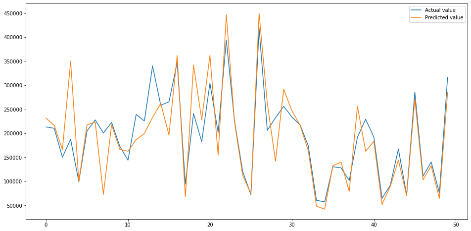
Assess the top performing model
Next, we’ll fit the the XGBRegressor() model to the data using its default parameters and plot the performance of the predictions against the actual values. As you can see, this is already looking pretty good. The tuning step might shave a bit more off the RMSE.
regressor = XGBRegressor()
model = regressor.fit(X_train, y_train)
y_pred = model.predict(X_test)
test = pd.DataFrame({'Predicted value':y_pred, 'Actual value':y_test})
fig= plt.figure(figsize=(16,8))
test = test.reset_index()
test = test.drop(['index'],axis=1)
plt.plot(test[:50])
plt.legend(['Actual value','Predicted value'])
<matplotlib.legend.Legend at 0x7fc9b5d20940>
Tune the model’s hyperparameters
To tune the XGBRegressor() model (or any Scikit-Learn compatible model) the first step is to determine which hyperparameters are available for tuning. You can view these by printing model.get_params(), however, you’ll likely need to check the documentation for the selected model to determine how they can be tuned.
model.get_params()
{'objective': 'reg:squarederror',
 'base_score': 0.5,
 'booster': 'gbtree',
 'colsample_bylevel': 1,
 'colsample_bynode': 1,
 'colsample_bytree': 1,
 'gamma': 0,
 'gpu_id': -1,
 'importance_type': 'gain',
 'interaction_constraints': '',
 'learning_rate': 0.300000012,
 'max_delta_step': 0,
 'max_depth': 6,
 'min_child_weight': 1,
 'missing': nan,
 'monotone_constraints': '()',
 'n_estimators': 100,
 'n_jobs': 0,
 'num_parallel_tree': 1,
 'random_state': 0,
 'reg_alpha': 0,
 'reg_lambda': 1,
 'scale_pos_weight': 1,
 'subsample': 1,
 'tree_method': 'exact',
 'validate_parameters': 1,
 'verbosity': None}
Next, take a small selection of the hyperparameters and add them to a dict() and assign this to the param_grid. We’ll then define the model and configure the GridSearchCV function to test each unique combination of hyperparameters and record the neg_root_mean_squared_error on each iteration. After going through the whole batch, the optimum model parameters can be printed.
param_grid = dict(
    n_jobs=[16],
    learning_rate=[0.1, 0.5],
    objective=['reg:squarederror'],
    max_depth=[5, 10, 15],
    n_estimators=[100, 500, 1000],
    subsample=[0.2, 0.8, 1.0],
    gamma=[0.05, 0.5],
    scale_pos_weight=[0, 1],
    reg_alpha=[0, 0.5],
    reg_lambda=[1, 0],
)

model = XGBRegressor(random_state=1, verbosity=1)

grid_search = GridSearchCV(estimator=model,
                           param_grid=param_grid,
                           scoring='neg_root_mean_squared_error',
                           )

best_model = grid_search.fit(X_train, y_train)
print('Optimum parameters', best_model.best_params_)
Optimum parameters {'gamma': 0.05, 'learning_rate': 0.1, 'max_depth': 5,
'n_estimators': 1000, 'n_jobs': 16, 'objective': 'reg:squarederror',
 'reg_alpha': 0, 'reg_lambda': 1, 'scale_pos_weight': 0, 'subsample': 0.8}
Obviously, the more values you add to the param_grid the more iterations GridSearchCV() will conduct, and this can greatly increase the run-time. To reduce this, it’s wise to add a few to start with and then add other values on either side until you improve the result.
Fit the best model
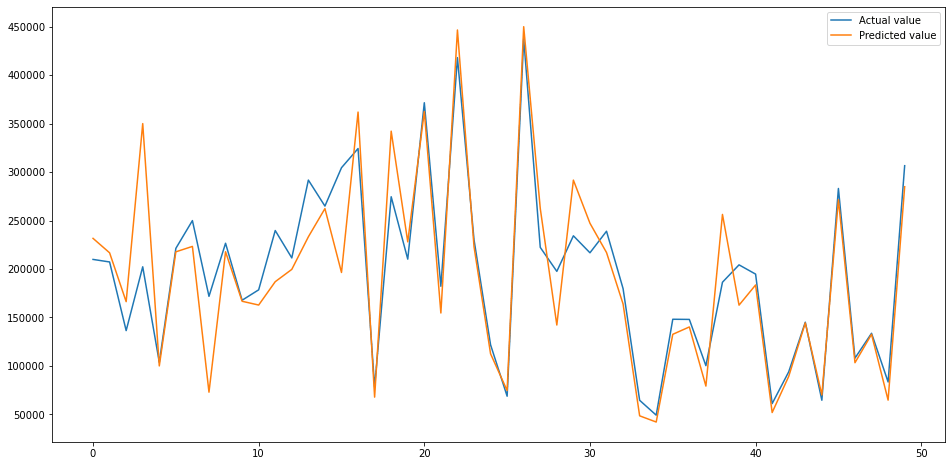
Finally, take the optimum parameters identified by GridSearchCV and add them to the XGBRegressor() model and re-fit it to your training data, generating new predictions from the test data and assess the mean squared error.
The hyperparameter tuning step has further improved the RMSE, taking it from 44041 to 42040. Compared to our initial model, that’s an overall improvement of 39% from 69076 to 42040.
regressor = XGBRegressor(
    gamma=0,
    learning_rate=0.1,
    max_depth=5,
    n_estimators=1000,
    n_jobs=16,
    objective='reg:squarederror',
    subsample=0.8,
    scale_pos_weight=0,
    reg_alpha=0,
    reg_lambda=1
)
model = regressor.fit(X_train, y_train)
y_pred = model.predict(X_test)

np.sqrt(mean_squared_error(y_test, y_pred))
42040.78739303113
test = pd.DataFrame({'Predicted value':y_pred, 'Actual value':y_test})
fig= plt.figure(figsize=(16,8))
test = test.reset_index()
test = test.drop(['index'],axis=1)
plt.plot(test[:50])
plt.legend(['Actual value','Predicted value'])
<matplotlib.legend.Legend at 0x7fc9b5d6a7c0>
Matt Clarke, Saturday, March 06, 2021


Other posts you might like

How to tune a LightGBMClassifier model with Optuna
The LightGBM model is a gradient boosting framework that uses tree-based learning algorithms, much like the popular XGBoost model. LightGBM supports both classification and regression tasks, and is known for...

How to create a customer retention model with XGBoost
Although all business know the importance of retaining customers, few companies are actually able to measure customer retention accurately, and fewer still can predict which ones will churn or be...
