How to assign RFM scores with quantile-based discretization
Use quantile-based discretization and K-means clustering to calculate RFM scores to your customers based on recency, frequency, and monetary value.

RFM segmentation is one of the oldest and most effective ways to segment customers. RFM models are based on three simple values - recency, frequency, and monetary value - which define for each customer how long it’s been since their last order, how many times they’ve purchased, and how much they’ve spent.
These three simple metrics are extremely powerful in predicting future customer behaviour and allow you to visualise their differences when segmented.
By binning the raw RFM metrics into quintiles from 1-5, you can create individual scores that allow you to compare each customer’s recency, frequency, and monetary value to those of others. Customers who have shopped recently get a 5, while those who’ve not been seen for a long time get a 1. Customers who have made lots of orders get a 5 for frequency, while those who’ve placed a single order are assigned a 1. Customers who’ve spent the most get a 5 for monetary, while those who’ve spent the least get a 1.
In combination, the three digit RFM scores cover 125 different states from 111 (least recency, lowest frequency, lowest monetary value) to 555 (most recent, highest frequency, highest monetary value) allowing marketers and sales staff to understand where a customer sits in relation to others without needing to see or analyse the raw data of potentially tens of thousands of other people.
While it’s an old methodology, RFM is still 100% valid today and is still subject to new research. Just this year a number of new papers on RFM have been published which document some of the processes savvy retailers are using.
We’re going to tackle one of these new approaches to assigning RFM scores here by comparing the use of the standard quantile-based discretization approach to the use of K-mean clustering and K-means clustering with an additional log transformation.
Load the packages
For this project we’ll be using Pandas and Numpy for data manipulation, the KMeans model from the Scikit Learn cluster package, and Seaborn for creating some simple charts to visualise the statistical distribution of our data.
import pandas as pd
import numpy as np
import seaborn as sns
from sklearn.cluster import KMeans
Load your transactional data
You don’t need particularly sophisticated raw data in order to calculate the underlying recency, frequency, and monetary metrics. They’re based on standard transactional data which needs to comprise the customer ID, the order ID, the total order revenue, and the date the order was placed. Load your data into a Pandas dataframe and set your order date field to datetime format.
df = pd.read_csv('orders.csv', low_memory=False)
df = df[['order_id','customer_id','total_revenue','date_created']]
df['date_created'] = pd.to_datetime(df['date_created'])
df.head(3)
| order_id | customer_id | total_revenue | date_created | |
|---|---|---|---|---|
| 0 | 299527 | 166958 | 74.01 | 2017-04-07 05:54:37 |
| 1 | 299528 | 191708 | 44.62 | 2017-04-07 07:32:54 |
| 2 | 299529 | 199961 | 16.99 | 2017-04-07 08:18:45 |
Create a dataframe of unique customers
As RFM is a customer-level metric, we next need to create a dataframe of unique customers from our initial transactional dataset. We can do this using the Pandas unique() function to select only the unique customer_id values and then rename the column accordingly.
df_customers = pd.DataFrame(df['customer_id'].unique())
df_customers.columns = ['customer_id']
df_customers.head()
| customer_id | |
|---|---|
| 0 | 166958 |
| 1 | 191708 |
| 2 | 199961 |
| 3 | 199962 |
| 4 | 199963 |
Calculate customer recency
Recency is a measure of the number of days since the customer last placed an order. Therefore, to calculate this we need to first identify the date of their most recent transaction, which we can do using df.groupby('customer_id')['date_created'].max().reset_index(). Once we’ve got that we can calculate the timedelta between the current datetime and the date of their last order and return the number of days that have elapsed.
df_recency = df.groupby('customer_id')['date_created'].max().reset_index()
df_recency.columns = ['customer_id','recency_date']
df_customers = df_customers.merge(df_recency, on='customer_id')
df_customers['recency'] = round((pd.to_datetime('today') - df_customers['recency_date'])\
                                / np.timedelta64(1, 'D') ).astype(int)
Calculate order frequency
Order frequency is simply the number of orders each customer has placed. This is easy to calculate. Just groupby() the customer_id column and return the number of unique values in the order_id column.
df_frequency = df.groupby('customer_id')['order_id'].nunique().reset_index()
df_frequency.columns = ['customer_id','frequency']
df_customers = df_customers.merge(df_frequency, on='customer_id')
Calculate monetary value
The monetary value column is simply the sum() of the total_revenue column for each customer. (Some researchers do favour the mean() of the total_revenue or the AOV, so feel free to try this approach.) Calculate the value and then merge it back onto the customers dataframe. I’ve saved my processed data to a separate file so I can use it elsewhere, but you can skip this if you don’t need it.
df_monetary = df.groupby('customer_id')['total_revenue'].sum().reset_index()
df_monetary.columns = ['customer_id','monetary']
df_customers = df_customers.merge(df_monetary, on='customer_id')
df_customers.head()
| customer_id | recency_date | recency | frequency | monetary | |
|---|---|---|---|---|---|
| 0 | 166958 | 2019-12-18 06:01:18 | 315 | 5 | 188.92 |
| 1 | 191708 | 2020-04-11 07:49:24 | 199 | 15 | 683.79 |
| 2 | 199961 | 2017-04-07 08:18:45 | 1299 | 1 | 16.99 |
| 3 | 199962 | 2017-04-07 08:20:00 | 1299 | 1 | 11.99 |
| 4 | 199963 | 2017-04-07 08:21:34 | 1299 | 1 | 14.49 |
df_customers.to_csv('raw_rfm_metrics.csv', index=False)
Examine the statistical distributions
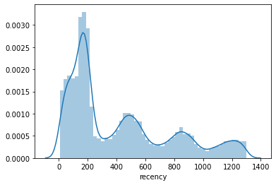
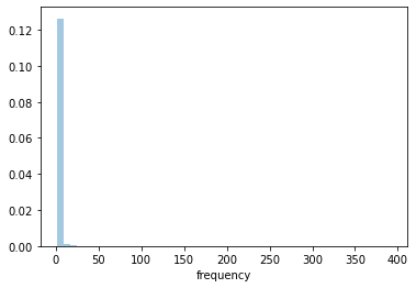
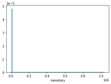
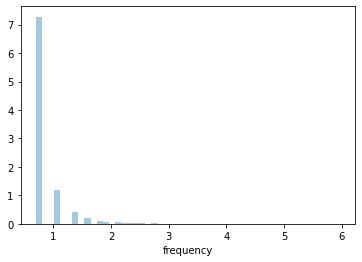
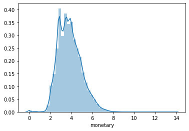
Next we’ll use Seaborn to plot the statistical distributions of the recency, frequency, and monetary data. The frequency and monetary values are heavily skewed, but the recency is far less so. As this retailer has strong seasonality, there are some interesting curves in the slope. As you might imagine, this introduces some challenges, which we’ll see later.
ax = sns.distplot(df_customers['recency'])
ax = sns.distplot(df_customers['frequency'])
ax = sns.distplot(df_customers['monetary'])
Calculating RFM scores using quantile-based discretization
Calculate the R score
For recency, customers with a lower recency are more valuable than those with a higher recency. For example, someone who shopped 7 days ago is far more likely to be a customer than someone last seen 1298 days ago. As a result, we score these differently to the frequency and monetary labels. To create five approximately equal segments of customers we’ll apply qcut() to the recency column and assign labels from 5 to 1.
df_customers['r'] = pd.qcut(df_customers['recency'], q=5, labels=[5, 4, 3, 2, 1])
If you run an aggregation and group the data by the r score and count the number of customers and their minimum, maximum, and mean recency, you’ll see some clear splits in the data. The ones with a score of 5 are very recent, last seen between 6 and 122 days ago, while those with a score of 1 were last seen 776 to 1298 days ago.
df_customers.groupby('r').agg(
    count=('customer_id', 'count'),
    min_recency=('recency', min),
    max_recency=('recency', max),
    std_recency=('recency', 'std'),
    avg_recency=('recency', 'mean')
).sort_values(by='avg_recency')
| count | min_recency | max_recency | std_recency | avg_recency | |
|---|---|---|---|---|---|
| r | |||||
| 5 | 36371 | 7 | 123 | 32.914273 | 66.371367 |
| 4 | 36185 | 124 | 189 | 18.027304 | 160.338428 |
| 3 | 35768 | 190 | 436 | 82.832877 | 278.756794 |
| 2 | 36058 | 437 | 776 | 92.764614 | 562.302263 |
| 1 | 36076 | 777 | 1299 | 163.633135 | 1013.147078 |
Calculate the M score
Since a higher monetary value is a better thing for the business, we score customers here from 1 to 5. Those who spend the most get a five and those who spend the least get a 1. We can use the same approach for qcut() and just switch the direction of the labels.
df_customers['m'] = pd.qcut(df_customers['monetary'], q=5, labels=[1, 2, 3, 4, 5])
Generating the grouped statistics for the monetary score shows us that customers with a score of 1 have spent between zero (presumably because they returned or canceled their order) and £16.87, while those with a score of 5 have spent between £114.99 and £1,036,590. Clearly, there’s a big difference between the spends of some of the customers.
df_customers.groupby('m').agg(
    count=('customer_id', 'count'),
    min_monetary=('monetary', min),
    max_monetary=('monetary', max),
    std_monetary=('monetary', 'std'),
    avg_monetary=('monetary', 'mean')
).sort_values(by='avg_monetary')
| count | min_monetary | max_monetary | std_monetary | avg_monetary | |
|---|---|---|---|---|---|
| m | |||||
| 1 | 36096 | 0.00 | 16.87 | 3.545414 | 11.714210 |
| 2 | 36087 | 16.88 | 31.35 | 4.336020 | 23.365174 |
| 3 | 36095 | 31.36 | 54.42 | 6.821548 | 41.994196 |
| 4 | 36106 | 54.43 | 114.99 | 17.146486 | 79.267260 |
| 5 | 36074 | 114.99 | 1036590.86 | 5497.076346 | 353.171247 |
This really highlights the potential drawback of using quantile-based discretization on skewed data. While monetary scores from 1 to 4 show low standard deviations, the standard deviation in the 5 segment is so vast that it makes the segment almost unusable by marketers. While the segments have been created in the recommended manner, this shows we sometimes need to use an alternative approach to binning based on the underlying statistical distributions in the data.
Calculate the F score
Using qcut() quantile-based discretization to create frequency scores is more challenging because the typical spread of order volumes means that bin edges may overlap. If you experience this, qcut() will throw an error telling you “ValueError: Bin edges must be unique” and that you can “You can drop duplicate edges by setting the ‘duplicates’ kwarg”. You can avoid this by appending .rank(method='first').
df_customers['f'] = pd.qcut(df_customers['frequency'].rank(method='first'), q=5, labels=[1, 2, 3, 4, 5])
df_customers.head()
| customer_id | recency_date | recency | frequency | monetary | r | m | f | |
|---|---|---|---|---|---|---|---|---|
| 0 | 166958 | 2019-12-18 06:01:18 | 315 | 5 | 188.92 | 3 | 5 | 5 |
| 1 | 191708 | 2020-04-11 07:49:24 | 199 | 15 | 683.79 | 3 | 5 | 5 |
| 2 | 199961 | 2017-04-07 08:18:45 | 1299 | 1 | 16.99 | 1 | 2 | 1 |
| 3 | 199962 | 2017-04-07 08:20:00 | 1299 | 1 | 11.99 | 1 | 1 | 1 |
| 4 | 199963 | 2017-04-07 08:21:34 | 1299 | 1 | 14.49 | 1 | 1 | 1 |
However, as with the monetary data, we encounter another issue with quantile-based discretization for calculating RFM scores on skewed data. It gives you lovely equal group sizes, but the scores don’t make a lot of sense because the frequency is heavily skewed resulting in a really long and quite useless tail.
df_customers.groupby('f').agg(
    count=('customer_id', 'count'),
    min_frequency=('frequency', min),
    max_frequency=('frequency', max),
    std_frequency=('frequency', 'std'),
    avg_frequency=('frequency', 'mean')
).sort_values(by='avg_frequency')
| count | min_frequency | max_frequency | std_frequency | avg_frequency | |
|---|---|---|---|---|---|
| f | |||||
| 1 | 36092 | 1 | 1 | 0.000000 | 1.000000 |
| 2 | 36091 | 1 | 1 | 0.000000 | 1.000000 |
| 3 | 36092 | 1 | 1 | 0.000000 | 1.000000 |
| 4 | 36091 | 1 | 2 | 0.364138 | 1.157352 |
| 5 | 36092 | 2 | 392 | 4.383576 | 3.697218 |
Create the RFM segment
Finally, we can concatenate the r, f, and m values in a single column to create the RFM score for each customer. If you print out the head() of your df_customers dataframe you’ll see the raw recency, frequency, and monetary values for each customers alongside their scores.
df_customers['rfm'] = df_customers['r'].astype(str) +\
                      df_customers['f'].astype(str) +\
                      df_customers['m'].astype(str)
Create the aggregate RFM score
You can also calculate additional aggregate metrics, such as the RFM score (recency + frequency + monetary) and use weightings to give certain variables, such as recency more impact than monetary. I tend to find that the individual values get used most, as the rfm_score metric obviously conceals some detail, however, it can be useful for quick sorting.
df_customers['rfm_score'] = df_customers['r'].astype(int) +\
                            df_customers['f'].astype(int) +\
                            df_customers['m'].astype(int)
df_customers.head()
| customer_id | recency_date | recency | frequency | monetary | r | m | f | rfm | rfm_score | |
|---|---|---|---|---|---|---|---|---|---|---|
| 0 | 166958 | 2019-12-18 06:01:18 | 315 | 5 | 188.92 | 3 | 5 | 5 | 355 | 13 |
| 1 | 191708 | 2020-04-11 07:49:24 | 199 | 15 | 683.79 | 3 | 5 | 5 | 355 | 13 |
| 2 | 199961 | 2017-04-07 08:18:45 | 1299 | 1 | 16.99 | 1 | 2 | 1 | 112 | 4 |
| 3 | 199962 | 2017-04-07 08:20:00 | 1299 | 1 | 11.99 | 1 | 1 | 1 | 111 | 3 |
| 4 | 199963 | 2017-04-07 08:21:34 | 1299 | 1 | 14.49 | 1 | 1 | 1 | 111 | 3 |
Examining the mean_recency, mean_frequency, and mean_monetary for each of the RFM scores from 3 to 15 gives a really nice picture of our customers. The lowest scoring customers with an rfm_score of 3 who are in the rfm_segment 111 have a mean recency of 991 days, have placed a single order and spent an average of £11.
The top customers in the rfm_score 15 group and the rfm_segment 555 have been seen 61 days ago, have placed an average of 5.7 orders and spent £591. Marketers can clearly see who to target with reactivation campaigns and who they should be giving preferential treatment to ensure they don’t churn.
df_customers.groupby('rfm_score').agg(
    customers=('customer_id', 'count'),
    mean_recency=('recency', 'mean'),
    mean_frequency=('frequency', 'mean'),
    mean_monetary=('monetary', 'mean'),
).sort_values(by='rfm_score')
| customers | mean_recency | mean_frequency | mean_monetary | |
|---|---|---|---|---|
| rfm_score | ||||
| 3 | 7356 | 991.781403 | 1.000000 | 11.002807 |
| 4 | 8195 | 980.658694 | 1.000000 | 22.480073 |
| 5 | 14741 | 784.199986 | 1.000000 | 26.762419 |
| 6 | 15797 | 701.943913 | 1.007660 | 43.556238 |
| 7 | 18184 | 530.294985 | 1.020568 | 70.994995 |
| 8 | 18173 | 343.364277 | 1.046828 | 44.141714 |
| 9 | 17427 | 327.299420 | 1.134045 | 64.289315 |
| 10 | 17807 | 256.091200 | 1.222104 | 63.773739 |
| 11 | 16690 | 237.216058 | 1.473697 | 77.827959 |
| 12 | 15278 | 222.878125 | 1.836890 | 127.955221 |
| 13 | 12732 | 157.297204 | 2.385171 | 168.094980 |
| 14 | 9718 | 103.189648 | 2.794814 | 241.868315 |
| 15 | 8360 | 61.600478 | 5.739234 | 591.236373 |
Overcoming skewness when calculating RFM scores
As we’ve seen above, using quantile-based discretization for the creation of RFM segments on a highly skewed dataset can cause some issues. There are a few things that you can do to work around this. If it makes sense to do so, you could simply remove the outliers (those massive customers likely need preferential treatment anyway), or you could log transform the data before binning. However, there are two more common approaches:
Option 1: Use a time constraint
The easiest option would be to calculate the RFM metrics over a shorter period so the level of skewness is greatly reduced. For example, we could limit our scoring to just those customers who purchased in the last two years the standard deviation will drop massively. However, while this is commonly used, it does leave you with only a fraction of your customers with scores assigned and makes targeting lapsed customers much trickier.
Option 2: Use unequal binning
The other approach, and the one I prefer, is to use unequal binning. While the standard method of RFM scoring is to create equal bins with up to 125 quintiles from 111 to 555, in most cases they’re only used to get a basic understanding of the customers for targeting purposes.
The scores themselves are not generally used as model features, we use the raw data instead, so the sizes of the bins may not really matter that much. For practical marketing purposes, I think it’s better to have usable bins than full bins. K-means clustering is becoming one of the most popular ways to perform this binning on such datasets, and has been covered in several papers recently.

K-means clustering
When you’re using unequal binning on RFM data there are a number of different algorithms you can apply. One of the
simplest is to use define the bounds for each binning using cut(), but this would mean we’d need to adjust our code as the customer base changed. To avoid that, we could either manually calculate the bounds using percentiles to automatically create dynamic bin edges, or we could use the Fisher-Jenks algorithm to determine the natural bounds and then pass those values into cut().
However, the easiest option is to use an unsupervised clustering algorithm such as K-means and let it figure things out using each of the raw RFM metrics. K-means clustering is a good choice for solving the problem of skewness we experienced in this data set. However, there’s an important factor to remember when using it for binning RFM scores.
Ordinarily, the labels assigned to K-means clusters aren’t important, but in RFM segmentation they need to denote the correct ordering of the data. As a result, we need to sort them, and ensure the recency sort order gives higher scores to lower values, and the frequency and monetary sorting gives higher scores to higher values. Here’s why:
df_clusters = df_customers[['recency']]

kmeans = KMeans(n_clusters=5)
kmeans.fit(df_clusters)
KMeans(n_clusters=5)
As you can see from the data below, if you fit a KMeans model to the recency column data and don’t sort it, the cluster numbers assigned don’t follow the average recency of each cluster. The cluster with the lowest recency would be R=1 in RFM terms, but occupies position 3 of the index. We need to sort the data like this then reassign the correct segment to each clustered customer.
df_clusters = df_clusters.assign(cluster=kmeans.labels_)
df_clusters.groupby('cluster')['recency'].mean().sort_values(ascending=False).to_frame()
| recency | |
|---|---|
| cluster | |
| 2 | 1172.660823 |
| 1 | 839.627699 |
| 4 | 497.569594 |
| 0 | 196.813082 |
| 3 | 73.539744 |
Sorting K-means clusters
It’s a bit of a ball-ache to sort the K-Means clusters so they’re in the right order. To achieve this I wrote the function below. It’s a bit complex but it basically lets you fit a K-Means model to a given metric column (i.e. recency, frequency, or monetary), clusters the data and then re-order it so the cluster label (i.e. 1-5) matches the mean distribution of the metric within the dataset.
Since recency is sorted the opposite way to frequency and monetary (because lower recency is better, while higher frequency/monetary are better), it also handles sort order and lets you log+1 transform the data to handle skewed statistical distributions. There’s probably a more elegant and less hacky solution to this quick version, so please let me know in the comments if you know one!
def sorted_kmeans(df, metric_column, cluster_name, ascending=True, log=False):
    """Runs a K-means clustering algorithm on a specific metric column
    in a Pandas dataframe; sorts the data in a specified direction; and
    reassigns cluster numbers to match the data distribution, so they
    are appropriate for RFM segmentation. Includes a log+1 transformation
    for heavily skewed datasets.

    :param df: Pandas dataframe containing RFM data
    :param metric_column: Column name of metric to cluster, i.e. 'recency'
    :param cluster_name: Name to assign to clustered metric, i.e. 'R'
    :param ascending: Sort ascending (M and F), or descending (R)
    :return
        Original Pandas dataframe with additional column
    """

    if log:
        df[metric_column] = np.log(df[metric_column]+1)

    # Fit the model
    kmeans = KMeans(n_clusters=5)
    kmeans.fit(df[[metric_column]])

    # Assign the initial unsorted cluster
    initial_cluster = 'unsorted_'+cluster_name
    df[initial_cluster] = kmeans.predict(df[[metric_column]])+1
    df[cluster_name] = df[initial_cluster]

    # Group the clusters and re-rank to determine the correct order
    df_sorted = df.groupby(initial_cluster)[metric_column].mean().round(2).reset_index()
    df_sorted = df_sorted.sort_values(by=metric_column, ascending=ascending).reset_index(drop=True)
    df_sorted[cluster_name] = df_sorted[metric_column].rank(method='max', ascending=ascending).astype(int)

    # Merge data and drop redundant columns
    df = df.merge(df_sorted[[cluster_name, initial_cluster]], on=[initial_cluster])
    df = df.drop(initial_cluster, axis=1)
    df = df.drop(cluster_name+'_x', axis=1)
    df = df.rename(columns={cluster_name+'_y':cluster_name})

    return df
To create the RFM segments using K-means clustering we can simply run the function three times, and assign the resulting dataframe back to the function so it adds the next value to the data. As I’ve not defined the log argument, the data here aren’t being log transformed.
df_customers = sorted_kmeans(df_customers, 'recency', 'R', ascending=False)
df_customers = sorted_kmeans(df_customers, 'frequency', 'F', ascending=True)
df_customers = sorted_kmeans(df_customers, 'monetary', 'M', ascending=True)
df_customers.head()
| customer_id | recency_date | recency | frequency | monetary | r | m | f | rfm | rfm_score | R | F | M | |
|---|---|---|---|---|---|---|---|---|---|---|---|---|---|
| 0 | 166958 | 2019-12-18 06:01:18 | 315 | 5 | 188.92 | 3 | 5 | 5 | 355 | 13 | 4 | 2 | 1 |
| 1 | 12052 | 2020-03-20 18:35:15 | 221 | 3 | 208.59 | 3 | 5 | 5 | 355 | 13 | 4 | 2 | 1 |
| 2 | 199983 | 2020-02-20 14:17:46 | 250 | 3 | 61.20 | 3 | 4 | 5 | 354 | 12 | 4 | 2 | 1 |
| 3 | 199994 | 2020-05-20 10:07:15 | 160 | 5 | 202.69 | 4 | 5 | 5 | 455 | 14 | 4 | 2 | 1 |
| 4 | 200003 | 2020-04-15 14:31:19 | 195 | 3 | 93.87 | 3 | 4 | 5 | 354 | 12 | 4 | 2 | 1 |
Examining the statistics for the R segment shows we’ve got a lot of fairly recent customers, indicating that this company is doing well acquisition and customer retention wise. There’s plenty of data in each segment to allow marketers enough data to make their reactivation campaigns viable.
df_customers.groupby('R').agg(
    customers=('customer_id', 'count'),
    min_recency=('recency', min),
    max_recency=('recency', max),
    std_recency=('recency', 'std'),
    avg_recency=('recency', 'mean')
).sort_values(by='avg_recency')
| customers | min_recency | max_recency | std_recency | avg_recency | |
|---|---|---|---|---|---|
| R | |||||
| 5 | 41012 | 7 | 136 | 36.946592 | 73.539744 |
| 4 | 57836 | 137 | 348 | 47.805535 | 196.975154 |
| 3 | 39562 | 349 | 669 | 77.355098 | 498.059653 |
| 2 | 25359 | 670 | 1007 | 82.002497 | 840.557632 |
| 1 | 16689 | 1008 | 1299 | 77.827297 | 1173.467374 |
The statistics for F show that a huge number of customers have only placed one order, which is something that’s very common in ecommerce. The customers with a score of 5 for frequency are very different from the others and have much higher average frequencies.
df_customers.groupby('F').agg(
    customers=('customer_id', 'count'),
    min_frequency=('frequency', min),
    max_frequency=('frequency', max),
    std_frequency=('frequency', 'std'),
    avg_frequency=('frequency', 'mean')
).sort_values(by='avg_frequency')
| customers | min_frequency | max_frequency | std_frequency | avg_frequency | |
|---|---|---|---|---|---|
| F | |||||
| 1 | 161526 | 1 | 2 | 0.348430 | 1.141395 |
| 2 | 15263 | 3 | 6 | 0.979677 | 3.787067 |
| 3 | 3190 | 7 | 15 | 2.274094 | 9.277743 |
| 4 | 473 | 16 | 87 | 8.262115 | 22.012685 |
| 5 | 6 | 145 | 392 | 96.099254 | 218.333333 |
Finally, the M score shows a similar picture to F, due to all those single-order customers, while at the opposite end of the spectrum we’ve got one massively lucrative customer who generates a metric shit-tonne of revenue. We end up with segments that better indicate the value of the customers to the business, but which are obviously rather unequal in size.
df_customers.groupby('M').agg(
    customers=('customer_id', 'count'),
    min_monetary=('monetary', min),
    max_monetary=('monetary', max),
    std_monetary=('monetary', 'std'),
    avg_monetary=('monetary', 'mean')
).sort_values(by='avg_monetary')
| customers | min_monetary | max_monetary | std_monetary | avg_monetary | |
|---|---|---|---|---|---|
| M | |||||
| 1 | 172489 | 0.00 | 374.42 | 68.218285 | 6.431079e+01 |
| 2 | 7766 | 374.46 | 2227.00 | 351.353277 | 6.868829e+02 |
| 3 | 199 | 2238.25 | 20096.58 | 2601.816439 | 3.791054e+03 |
| 4 | 3 | 41940.85 | 78970.38 | 20562.845756 | 5.529054e+04 |
| 5 | 1 | 1036590.86 | 1036590.86 | NaN | 1.036591e+06 |

Applying log transformation
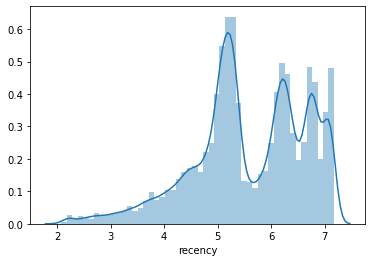
The final approach is to use K-means clustering for the creation of the segments, but to also apply a log+1 transformation to the metrics to handle the skewness in the dataset. This gives us segments which fall somewhere between the quantile-based discretization approach and the regular non-transformed K-means, so that looks to be the best approach for this company. You can also try using StandardScaler() to see if this improves performance, as K-means does expect equal variance.
Recency via K-means with log+1 transformation
clusters_log = sorted_kmeans(df_customers, 'recency', 'R', ascending=False, log=True)
clusters_log.head()
| customer_id | recency_date | recency | frequency | monetary | r | m | f | rfm | rfm_score | F | M | R | |
|---|---|---|---|---|---|---|---|---|---|---|---|---|---|
| 0 | 166958 | 2019-12-18 06:01:18 | 5.755742 | 5 | 188.92 | 3 | 5 | 5 | 355 | 13 | 2 | 1 | 2 |
| 1 | 2019 | 2019-12-20 17:18:29 | 5.746203 | 4 | 187.54 | 3 | 5 | 5 | 355 | 13 | 2 | 1 | 2 |
| 2 | 200130 | 2019-12-06 14:36:49 | 5.789960 | 3 | 139.48 | 3 | 5 | 5 | 355 | 13 | 2 | 1 | 2 |
| 3 | 200395 | 2019-12-24 11:47:37 | 5.733341 | 4 | 147.78 | 3 | 5 | 5 | 355 | 13 | 2 | 1 | 2 |
| 4 | 196515 | 2019-12-29 17:07:22 | 5.717028 | 4 | 310.19 | 3 | 5 | 5 | 355 | 13 | 2 | 1 | 2 |
ax = sns.distplot(clusters_log['recency'])
clusters_log.groupby('R').agg(
    count=('customer_id', 'count'),
    min_recency=('recency', min),
    max_recency=('recency', max),
    std_recency=('recency', 'std'),
    avg_recency=('recency', 'mean')
).sort_values(by='avg_recency')
| count | min_recency | max_recency | std_recency | avg_recency | |
|---|---|---|---|---|---|
| R | |||||
| 5 | 9008 | 2.079442 | 3.663562 | 0.444930 | 3.084151 |
| 4 | 23923 | 3.688879 | 4.727388 | 0.291616 | 4.293835 |
| 3 | 61241 | 4.736198 | 5.659482 | 0.202653 | 5.167734 |
| 2 | 44296 | 5.662960 | 6.508769 | 0.200576 | 6.155100 |
| 1 | 41990 | 6.510258 | 7.170120 | 0.185897 | 6.864239 |
Frequency via K-means with log+1 transformation
clusters_log = sorted_kmeans(clusters_log, 'frequency', 'F', ascending=True, log=True)
clusters_log.head()
| customer_id | recency_date | recency | frequency | monetary | r | m | f | rfm | rfm_score | M | R | F | |
|---|---|---|---|---|---|---|---|---|---|---|---|---|---|
| 0 | 166958 | 2019-12-18 06:01:18 | 5.755742 | 1.791759 | 188.92 | 3 | 5 | 5 | 355 | 13 | 1 | 2 | 4 |
| 1 | 173791 | 2019-12-18 22:04:08 | 5.752573 | 1.791759 | 111.31 | 3 | 4 | 5 | 354 | 12 | 1 | 2 | 4 |
| 2 | 201608 | 2020-01-01 13:28:54 | 5.707110 | 1.791759 | 167.23 | 3 | 5 | 5 | 355 | 13 | 1 | 2 | 4 |
| 3 | 185842 | 2019-12-27 14:11:35 | 5.723585 | 1.945910 | 240.22 | 3 | 5 | 5 | 355 | 13 | 1 | 2 | 4 |
| 4 | 180212 | 2019-11-30 13:37:00 | 5.808142 | 1.791759 | 259.74 | 3 | 5 | 5 | 355 | 13 | 1 | 2 | 4 |
ax = sns.distplot(clusters_log['frequency'])
clusters_log.groupby('F').agg(
    count=('customer_id', 'count'),
    min_frequency=('frequency', min),
    max_frequency=('frequency', max),
    std_frequency=('frequency', 'std'),
    avg_frequency=('frequency', 'mean')
).sort_values(by='avg_frequency')
| count | min_frequency | max_frequency | std_frequency | avg_frequency | |
|---|---|---|---|---|---|
| F | |||||
| 1 | 138687 | 0.693147 | 0.693147 | 0.000000 | 0.693147 |
| 2 | 22839 | 1.098612 | 1.098612 | 0.000000 | 1.098612 |
| 3 | 11790 | 1.386294 | 1.609438 | 0.104155 | 1.457855 |
| 4 | 5445 | 1.791759 | 2.302585 | 0.171952 | 1.963479 |
| 5 | 1697 | 2.397895 | 5.973810 | 0.343545 | 2.702249 |
Monetary via K-means with log+1 transformation
clusters_log = sorted_kmeans(clusters_log, 'monetary', 'M', ascending=True, log=True)
clusters_log.head()
| customer_id | recency_date | recency | frequency | monetary | r | m | f | rfm | rfm_score | R | F | M | |
|---|---|---|---|---|---|---|---|---|---|---|---|---|---|
| 0 | 166958 | 2019-12-18 06:01:18 | 5.755742 | 1.791759 | 5.246603 | 3 | 5 | 5 | 355 | 13 | 2 | 4 | 4 |
| 1 | 173791 | 2019-12-18 22:04:08 | 5.752573 | 1.791759 | 4.721263 | 3 | 4 | 5 | 354 | 12 | 2 | 4 | 4 |
| 2 | 201608 | 2020-01-01 13:28:54 | 5.707110 | 1.791759 | 5.125332 | 3 | 5 | 5 | 355 | 13 | 2 | 4 | 4 |
| 3 | 185842 | 2019-12-27 14:11:35 | 5.723585 | 1.945910 | 5.485709 | 3 | 5 | 5 | 355 | 13 | 2 | 4 | 4 |
| 4 | 203929 | 2019-12-23 22:40:07 | 5.736572 | 1.791759 | 5.444709 | 3 | 5 | 5 | 355 | 13 | 2 | 4 | 4 |
ax = sns.distplot(clusters_log['monetary'])
clusters_log.groupby('M').agg(
    count=('customer_id', 'count'),
    min_monetary=('monetary', min),
    max_monetary=('monetary', max),
    std_monetary=('monetary', 'std'),
    avg_monetary=('monetary', 'mean')
).sort_values(by='avg_monetary')
| count | min_monetary | max_monetary | std_monetary | avg_monetary | |
|---|---|---|---|---|---|
| M | |||||
| 1 | 38717 | 0.000000 | 2.908539 | 0.385274 | 2.514048 |
| 2 | 46879 | 2.909084 | 3.676807 | 0.221237 | 3.306364 |
| 3 | 47001 | 3.677060 | 4.484696 | 0.227218 | 4.053475 |
| 4 | 34202 | 4.484809 | 5.539654 | 0.291592 | 4.924446 |
| 5 | 13659 | 5.539890 | 13.851449 | 0.541797 | 6.165789 |
Further reading
- Huang, Y., Zhang, M. and He, Y., 2020, June. Research on improved RFM customer segmentation model based on K-Means algorithm. In 2020 5th International Conference on Computational Intelligence and Applications (ICCIA) (pp. 24-27). IEEE.
- Gustriansyah, R., Suhandi, N. and Antony, F., 2020. Clustering optimization in RFM analysis based on k-means. Indones. J. Electr. Eng. Comput. Sci, 18(1), pp.470-477.
- Kabaskal, İ., 2020. Customer Segmentation Based On Recency Frequency Monetary Model: A Case Study in E-Retailing. International Journal of InformaticsTechnologies, 13(1).
- Miglautsch, J., 2002. Application of RFM principles: What to do with 1–1–1 customers?. Journal of Database Marketing & Customer Strategy Management, 9(4), pp.319-324.
Matt Clarke, Sunday, March 14, 2021


Other posts you might like

How to use the Pandas truncate() function
Have you ever needed to chop the top or bottom off a Pandas dataframe, or extract a specific section from the middle? If so, there’s a Pandas function called truncate()...

How to use Spacy for noun phrase extraction
Noun phrase extraction is a Natural Language Processing technique that can be used to identify and extract noun phrases from text. Noun phrases are phrases that function grammatically as nouns...
