How to perform a customer cohort analysis in Pandas
Customer cohort analysis examines differences between customers over time and is a powerful tool in guiding ecommerce acquisition strategy. Here's how it's done.

Cohort analysis is unlike most other customer segmentation techniques in that it typically uses a time-based element. It’s typically used to segment customers into groups, or cohorts, based on their acquisition date so that their behaviour can be examined over time.
For example, segmentation looks at customers at a given point in time, such as their current [RFM score] (/data-science/how-to-assign-rfm-scores-with-quantile-based-discretization). However, unlike the RFM model cohort analysis looks at a given metric at multiple points in time, allowing you to see how their behaviour changes.
While cohort analysis can be performed across the whole customer-base, it’s most powerful when it is combined with another segment or categorical variable so the behaviour of multiple cohorts can be compared.
My Master’s research, for example, studied how customers differed according to the level of discount they were given on their first order. Deep discounting meant customers were less likely to be retained, and the customers spent less and needed further big discounts to get them to repurchase.
Similarly, customers acquired via certain marketing channels, or through purchases of specific products or product categories, can differ markedly in their long-term business value, and cohort analysis can help you identify this and adapt your marketing strategy accordingly.
Analysing cohorts
Good cohort analysis usually starts with a business question. For example, my customer acquisition research was aiming to identify whether the company should use deep discounting via coupon codes to acquire new customers quickly and cheaply, or whether it should favour the slower and more expensive approach of using paid search advertising for new customer acquisition.
To perform this study, the first step was to assign customers to cohorts, and the second was to examine the behaviour of the cohorts over time. Cohorts can be constructed in several ways. The most common approach is to put all the customers acquired during a calendar month into a given “acquisition cohort”.
For future periods, various metrics can then be calculated over time, such as the number of orders placed, the AOV, or the number of items in each customer’s basket. However, cohorts are easy to create based on other factors, such as the marketing channel used, the level of discount offered, and countless other things. Here’s how it’s done.
Load the packages
Most cohort analysis work can be undertaken solely within Pandas, however, I’m also using the Python operator module for one function, and Seaborn and Matplotlib for some data visualisation. Anything you don’t have installed can be loaded into your environment using pip3 install packagename.
import pandas as pd
import operator as op
import seaborn as sns
import matplotlib.pyplot as plt
pd.set_option('max_columns', 10)
Load the data
Cohort analysis requires standard transactional data, that we can generate from a transactional item dataset. This needs to include the order_id, the customer_id and order_date, plus any metrics you wish to calculate.
The order_date column needs to a DateTime, which you can apply automatically when loading the data using the
parse_dates argument on read_csv(). As the functions I’ve written below specifically reference these column names, you might want to rename your dataframe columns to match.
df = pd.read_csv('transaction_items.csv', parse_dates=['order_date'])
df.head()
| order_id | sku | quantity | unit_price | customer_id | order_date | |
|---|---|---|---|---|---|---|
| 0 | 299527 | 1541255 | 1 | 22.94 | 166958.0 | 2017-04-07 04:55:58 |
| 1 | 299527 | 1052928 | 2 | 15.19 | 166958.0 | 2017-04-07 04:55:58 |
| 2 | 299527 | 1167973 | 1 | 20.69 | 166958.0 | 2017-04-07 04:55:58 |
| 3 | 299527 | 0 | 1 | 0.00 | 166958.0 | 2017-04-07 04:55:58 |
| 4 | 299528 | 2123242 | 2 | 22.31 | 191708.0 | 2017-04-07 06:34:07 |
Calculate the order cohort and acquisition cohort
For this simple demonstration of the process, our Pandas dataframe includes all customers acquired during a period. However, to modify this and select only those acquired via a specific channel during a period, all you need to do is add the appropriate categorical variable to your dataframe and filter accordingly before splitting the cohorts.
The acquisition cohort is a label which identifies the period during which each customer was acquired. Depending on the size of your dataset and the frequency at which your customers order, you might want to use monthly, quarterly, or yearly cohorts. The function below creates these for us.
By default, this uses a monthly cohort, so a customer ordering on 2017-04-07 04:55:58 would be placed in a cohort called 2017-04. If this was set to quarterly, they’d be placed in cohort 2017Q2. The new cohort labels get added to a DataFrame containing the unique customer_id, order_id, and order_date.
def get_cohorts(df, period='M'):
    """Given a Pandas DataFrame of transactional items, this function returns
    a Pandas DataFrame containing the acquisition cohort and order cohort which
    can be used for customer analysis or the creation of a cohort analysis matrix.

    Parameters
    ----------

    df: Pandas DataFrame
        Required columns: order_id, customer_id, order_date
    period: Period value - M, Q, or Y
        Create cohorts using month, quarter, or year of acquisition

    Returns
    -------
    products: Pandas DataFrame
        customer_id, order_id, order_date, acquisition_cohort, order_cohort
    """

    df = df[['customer_id','order_id','order_date']].drop_duplicates()
    df = df.assign(acquisition_cohort = df.groupby('customer_id')\
                   ['order_date'].transform('min').dt.to_period(period))
    df = df.assign(order_cohort = df['order_date'].dt.to_period(period))
    return df
df = get_cohorts(df, period='Q')
df.head()
| customer_id | order_id | order_date | acquisition_cohort | order_cohort | |
|---|---|---|---|---|---|
| 0 | 166958.0 | 299527 | 2017-04-07 04:55:58 | 2017Q2 | 2017Q2 |
| 4 | 191708.0 | 299528 | 2017-04-07 06:34:07 | 2017Q2 | 2017Q2 |
| 6 | 199961.0 | 299529 | 2017-04-07 07:18:50 | 2017Q2 | 2017Q2 |
| 8 | 199962.0 | 299530 | 2017-04-07 07:20:25 | 2017Q2 | 2017Q2 |
| 10 | 199963.0 | 299531 | 2017-04-07 07:21:40 | 2017Q2 | 2017Q2 |
Calculate the “retention” for each cohort
Next, we’ll create a function that counts how many of the customers acquired in a given cohort purchased again in subsequent periods. It’s common in cohort analysis to call this customer retention, but arguably it’s just a repurchase metric.
As with the above function, the period used can be modified using the period argument. This will create a Pandas
dataframe containing the count of
unique customers who purchased within each subsequent period. This is only handling counts, but you could easily change this to calculate revenue generated, AOV, or any other metrics you wish to measure.
def get_retention(df, period='M'):
    """Calculate the retention of customers in each month after their acquisition
    and return the count of customers in each month.

    Parameters
    ----------

    df: Pandas DataFrame
        Required columns: order_id, customer_id, order_date
    period: Period value - M, Q, or Y
        Create cohorts using month, quarter, or year of acquisition

    Returns
    -------
    products: Pandas DataFrame
        acquisition_cohort, order_cohort, customers, periods
    """

    df = get_cohorts(df, period).groupby(['acquisition_cohort', 'order_cohort'])\
                                .agg(customers=('customer_id', 'nunique')) \
                                .reset_index(drop=False)
    df['periods'] = (df.order_cohort - df.acquisition_cohort)\
    .apply(op.attrgetter('n'))

    return df
retention = get_retention(df)
retention.head()
| acquisition_cohort | order_cohort | customers | periods | |
|---|---|---|---|---|
| 0 | 2017-04 | 2017-04 | 3039 | 0 |
| 1 | 2017-04 | 2017-05 | 267 | 1 |
| 2 | 2017-04 | 2017-06 | 249 | 2 |
| 3 | 2017-04 | 2017-07 | 247 | 3 |
| 4 | 2017-04 | 2017-08 | 228 | 4 |
Create a cohort matrix
Next, we’ll use the above function to create a cohort matrix. This is a dataframe which shows each acquisition cohort on its own line and shows the number of customers who purchased in each subsequent period. If you set the percentage argument to True, the function will return the percentage of customers, instead of the raw numbers. As with the previous functions, these can be monthly, quarterly, or yearly.
def get_cohort_matrix(df, period='M', percentage=False):
    """Return a cohort matrix showing for each acquisition cohort, the number of
    customers who purchased in each period after their acqusition.

    Parameters
    ----------

    df: Pandas DataFrame
        Required columns: order_id, customer_id, order_date
    period: Period value - M, Q, or Y
        Create cohorts using month, quarter, or year of acquisition
    percentage: True or False
        Return raw numbers or a percentage retention

    Returns
    -------
    products: Pandas DataFrame
        acquisition_cohort, period
    """

    df = get_retention(df, period).pivot_table(index = 'acquisition_cohort',
                                               columns = 'periods',
                                               values = 'customers')

    if percentage:
        df = df.divide(df.iloc[:,0], axis=0)*100

    return df
Monthly cohorts
df_matrixm = get_cohort_matrix(df, 'M', percentage=True)
df_matrixm.head()
| periods | 0 | 1 | 2 | 3 | 4 | ... | 37 | 38 | 39 | 40 | 41 |
|---|---|---|---|---|---|---|---|---|---|---|---|
| acquisition_cohort | |||||||||||
| 2017-04 | 100.0 | 8.785785 | 8.193485 | 8.127674 | 7.502468 | ... | 6.646923 | 4.968740 | 4.540967 | 5.593945 | 0.822639 |
| 2017-05 | 100.0 | 7.972789 | 7.510204 | 7.210884 | 4.897959 | ... | 4.380952 | 3.809524 | 3.755102 | 0.380952 | NaN |
| 2017-06 | 100.0 | 6.605784 | 5.175038 | 5.022831 | 3.378995 | ... | 3.896499 | 3.500761 | 0.182648 | NaN | NaN |
| 2017-07 | 100.0 | 6.202261 | 4.155209 | 3.146960 | 2.505347 | ... | 3.452490 | 0.611060 | NaN | NaN | NaN |
| 2017-08 | 100.0 | 5.013550 | 3.387534 | 2.371274 | 1.524390 | ... | 0.474255 | NaN | NaN | NaN | NaN |
5 rows × 42 columns
Quarterly cohorts
df_matrixq = get_cohort_matrix(df, 'Q', percentage=True)
df_matrixq.head()
| periods | 0 | 1 | 2 | 3 | 4 | ... | 9 | 10 | 11 | 12 | 13 |
|---|---|---|---|---|---|---|---|---|---|---|---|
| acquisition_cohort | |||||||||||
| 2017Q2 | 100.0 | 15.381538 | 9.470947 | 8.290829 | 13.791379 | ... | 10.631063 | 5.790579 | 7.090709 | 12.141214 | 7.60076 |
| 2017Q3 | 100.0 | 7.271043 | 5.673266 | 8.683571 | 8.498321 | ... | 4.168114 | 5.082783 | 8.729883 | 5.198564 | NaN |
| 2017Q4 | 100.0 | 8.483290 | 7.415464 | 7.257267 | 6.209215 | ... | 4.844770 | 6.644255 | 3.816492 | NaN | NaN |
| 2018Q1 | 100.0 | 8.406794 | 6.536229 | 5.719200 | 5.848205 | ... | 6.600731 | 3.913137 | NaN | NaN | NaN |
| 2018Q2 | 100.0 | 6.980474 | 3.122347 | 3.641166 | 6.084332 | ... | 3.631733 | NaN | NaN | NaN | NaN |
5 rows × 14 columns
Annual cohorts
df_matrixy = get_cohort_matrix(df, 'Y', percentage=True)
df_matrixy.head()
| periods | 0 | 1 | 2 | 3 |
|---|---|---|---|---|
| acquisition_cohort | ||||
| 2017 | 100.0 | 21.685730 | 18.055966 | 15.202803 |
| 2018 | 100.0 | 14.173254 | 10.738102 | NaN |
| 2019 | 100.0 | 11.481330 | NaN | NaN |
| 2020 | 100.0 | NaN | NaN | NaN |
df_matrix = get_cohort_matrix(df, 'Y', percentage=False)
df_matrix.head()
| periods | 0 | 1 | 2 | 3 |
|---|---|---|---|---|
| acquisition_cohort | ||||
| 2017 | 23693.0 | 5138.0 | 4278.0 | 3602.0 |
| 2018 | 30741.0 | 4357.0 | 3301.0 | NaN |
| 2019 | 44028.0 | 5055.0 | NaN | NaN |
| 2020 | 69695.0 | NaN | NaN | NaN |
Creating cohort analysis heatmaps
Finally, we can create a heatmap to visualise our cohort. For each of the cohorts in our cohort matrix, this shows the percentage of the acquired customers who came back and purchased within a later period. Note that this isn’t the same as customer retention, which records the percentage of customers who came back up to a given period.
del df_matrixq[0]

f, ax = plt.subplots(figsize=(20, 5))
cmap = sns.color_palette("Blues")

monthly_sessions = sns.heatmap(df_matrixq,
                    annot=True,
                    linewidths=3,
                    ax=ax,
                    cmap=cmap,
                    square=False)

ax.axes.set_title("Cohort analysis",fontsize=20)
ax.set_xlabel("Acquisition cohort",fontsize=15)
ax.set_ylabel("Period",fontsize=15)
plt.show()
If you look at cohort 2017Q2, you’ll notice that customers acquired here are more likely to come back at the same point each year, implying that this is a valuable seasonal cohort to this business. The Q2 periods in future years don’t follow exactly the same pattern, so it would be worth investigating how these customers were acquired as they are behaving differently to the rest.
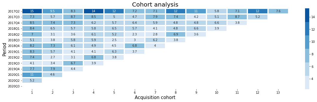
For this company, once this is known, it might be worth spending more on acquisitions during this period using the same technique, since more of the customers are likely to return than those acquired in other periods. It also shows that a single site-wide cohort analysis is really just the start, and that drilling-down through the data is often required using simple modifications of the process above.
Matt Clarke, Sunday, March 14, 2021


Other posts you might like

How to use the Pandas truncate() function
Have you ever needed to chop the top or bottom off a Pandas dataframe, or extract a specific section from the middle? If so, there’s a Pandas function called truncate()...

How to use Spacy for noun phrase extraction
Noun phrase extraction is a Natural Language Processing technique that can be used to identify and extract noun phrases from text. Noun phrases are phrases that function grammatically as nouns...
