How to create an ecommerce purchase intention model in Python
Ecommerce purchase intention models predict the probability of each customer making a purchase, so you can persuade those less likely to purchase using targeted offers. Here's how they work and how to build one.

Ecommerce purchase intention models analyse click-stream consumer behaviour data from web analytics platforms to predict whether a customer will make a purchase during their visit. These online shopping models are used to examine real time web analytics data and predict the probability of each customer making a purchase, so the retailer can serve a carefully targeted promotion to try and persuade those less likely to purchase.
The approach can avoid indiscriminately providing promotional discounts to customers who were going to purchase anyway, potentially training them to become more coupon-prone. According to recent research by Baati and Mohsil (2020), some online shopping retailers are also using the models to target basket or cart abandoners via email or telephone to try and persuade them to complete their purchase.
With a custom Google Analytics implementation, the technique could also be applied to the creation of custom audiences for Google Ads, which would allow the customers with a higher probability of converting to be targeted differently.
In this project, I’ll show you how you can create an ecommerce purchase intent model. It uses Google Analytics data to predict the probability that each customer will place an order, allowing you to target them with real-time offer popups, basket abandonment emails, paid search ads, or even telephone calls.
How do ecommerce purchase intention models work?
The simplest purchase intent models are classifiers, designed to analyse web analytics data and predict whether a customer will or won’t make a purchase during their visit. For example, in Baati and Mohsil’s model, they used Google Analytics online shopping data for full sessions and created a feature set based on a range of customer-based and session-based features to predict purchase intention from customer behaviour.
The concept is the same as that used in predictive lead scoring models, as well as sales response models.
| Feature | Description | Type |
|---|---|---|
| Day | Measures the closeness of the visit date to a key trading event. | Numerical |
| Operating system | The operating system used during the visit. | Categorical |
| Browser | The web browser used during the visit. | Categorical |
| Region | The geographic region of the visitor. | Categorical |
| Visitor type | Whether the customer was a new visitor or returning visitor. | Categorical |
| Weekend | A Boolean value indicating whether the visit fell on a weekend. | Categorical |
| Month | The month of the user's visit. | Categorical |
| Revenue | The target variable indicating whether the visit generated revenue. | Categorical |
These simple consumer behaviour metrics are potentially very powerful. By using these core features, engineering some new ones, and converting them to numeric representations, it’s possible to identify the correlation of the target variable to the individual web analytics metrics and predict each customer’s intention to purchase.
For example, customers from the site’s country who are using desktop browsers and shopping during the week might be much more likely to convert than people from abroad browsing via a mobile on the weekend. The purchase intention of customers who visit the site solely to view the returns page or report a damage is likely to be much lower than those who are viewing product pages and adding items to their shopping cart.
Although classification models are by far the most commonly used for predicting purchase intention from customer behaviour data, other researchers have used more sophisticated that use LSTM models or Markov models on sequential clickstream consumer behaviour data. The benefit of the latter is that they could work better on incomplete session data, rather than the full session data used here. The downside, is that they’re much more complex to implement.
Install the packages
First, open up a Jupyter notebook and install any packages you require. I’m using the NVIDIA Data Science Stack Docker container which uses the RAPIDS environment. This is pre-installed with a wide range of data science packages, so I only need to install a few things not included within the default stack. Any packages you don’t have installed can be installed via the Pip package manager like this:
!pip3 install lightgbm
!pip3 install imblearn
Load the packages
Next, import the packages below. Rather than just using a single classifier, we’re going to load up a bunch of them and test each one to see which gives us the best results. Since some models may throw ugly warnings, you may wish to disable the output of these by importing warnings and turning off the ConvergenceWarning.
import time
import pandas as pd
import numpy as np
import seaborn as sns
import matplotlib.pyplot as plt

from sklearn.model_selection import train_test_split
from sklearn.model_selection import cross_val_score
from sklearn.model_selection import GridSearchCV
from sklearn.feature_selection import SelectKBest
from sklearn.feature_selection import chi2
from imblearn.over_sampling import SMOTE
from imblearn.pipeline import Pipeline as imbpipeline
from sklearn.pipeline import Pipeline
from sklearn.compose import ColumnTransformer
from sklearn.impute import SimpleImputer
from sklearn.preprocessing import OneHotEncoder
from sklearn.preprocessing import OrdinalEncoder
from sklearn.preprocessing import StandardScaler
from sklearn.preprocessing import MinMaxScaler
from sklearn.metrics import accuracy_score
from sklearn.metrics import roc_auc_score
from sklearn.metrics import classification_report
from sklearn.metrics import confusion_matrix
from sklearn.metrics import f1_score
from sklearn.svm import SVC
from xgboost import XGBClassifier
from lightgbm import LGBMClassifier
from sklearn.dummy import DummyClassifier
from sklearn.neighbors import KNeighborsClassifier
from sklearn.tree import DecisionTreeClassifier
from sklearn.tree import ExtraTreeClassifier
from sklearn.ensemble import ExtraTreesClassifier
from sklearn.linear_model import RidgeClassifier
from sklearn.linear_model import SGDClassifier
from sklearn.ensemble import RandomForestClassifier
from sklearn.ensemble import AdaBoostClassifier
from sklearn.ensemble import BaggingClassifier
from sklearn.naive_bayes import BernoulliNB
from sklearn.neural_network import MLPClassifier
from warnings import simplefilter
from sklearn.exceptions import ConvergenceWarning
simplefilter("ignore", category=ConvergenceWarning)
Load the data
You can, of course, create your own purchase intention dataset if you wish. For demonstration purposes I’m using the online shopping dataset created by Sakar et al (2019) from their paper “Real-time prediction of online shoppers’ purchasing intention using multilayer perceptron and LSTM recurrent neural networks”. You can download this from Kaggle.
If you load the first three rows of data from the head() of the dataframe and then transpose the output using .T, you’ll be able to see what’s included. This consumer behaviour dataset is similar to the one used by Baati and Mohsil, but includes some additional features also extracted from Google Analytics. Some of these would have been extracted directly and then encoded, while other features have been engineered specifically based on the site examined. From these simple consumer behaviour metrics we should be able to calculate each customer’s intention to purchase.
df = pd.read_csv('online_shoppers_intention.csv')
df.sample(3).T
| 10435 | 6814 | 8045 | |
|---|---|---|---|
| Administrative | 4 | 0 | 4 |
| Administrative_Duration | 195.5 | 0 | 77.6667 |
| Informational | 0 | 0 | 0 |
| Informational_Duration | 0 | 0 | 0 |
| ProductRelated | 31 | 11 | 8 |
| ProductRelated_Duration | 1028.53 | 1197.8 | 159.75 |
| BounceRates | 0.0181818 | 0 | 0.0166667 |
| ExitRates | 0.0313131 | 0.01 | 0.0388889 |
| PageValues | 77.6648 | 0 | 0 |
| SpecialDay | 0 | 0 | 0 |
| Month | Nov | Oct | Nov |
| OperatingSystems | 3 | 2 | 3 |
| Browser | 2 | 2 | 2 |
| Region | 1 | 3 | 3 |
| TrafficType | 13 | 20 | 2 |
| VisitorType | Returning_Visitor | Returning_Visitor | Returning_Visitor |
| Weekend | False | False | False |
| Revenue | False | False | True |
Sakar et al created their consumer behaviour dataset from Google Analytics data from an online retail website. Each row of data in the dataset represents one of 12,330 sessions, of which 1908 led to a purchase. Rather than simply using all the sessions from a period, the authors restricted the data to include only one session per user.
They engineered a range of additional features by categorising the URLs visited into administrative, informational, and product related, and recorded the number of each page type visited, and the time spent on the pages. They also recorded the bounce rate, exit rate, and page value metrics from Google Analytics for each page. Like Baati and Mohsil, they also recorded the proximity to a special trading day, such as Mother’s Day, to help the model.
| Feature | Description |
|---|---|
| Administrative | Number of pages visited by the visitor about account management |
| Administrative duration | Total seconds spent viewing account management related pages |
| Informational | Number of informational pages visited by the visitor |
| Informational duration | Total seconds spent viewing informational pages |
| Product related | Number of product pages visited by the visitor |
| Product related duration | Total seconds spent viewing informational pages |
| Bounce rate | Average bounce rate value of the pages visited by visitor |
| Exit rate | Average exit rate value of the pages visited by visitor |
| Special day | Closeness of the visit date to a special trading day |
| Operating system | The operating system used on the visit |
| Browser | The browser used on the visit |
| Weekend | A Boolean value indicating whether the visit was on a weekend |
| Month | The month of the visit |
| Revenue | A class label indicating whether the customer purchased |
Feature engineering
While these steps are actually automated further down in our code, I’ll show you how you can achieve the same steps manually, so we can also examine the correlations of the features with the target variable. The data in the Sakar and Kostro dataset are already in pretty good shape, but there are a few things we need to do before we continue. The Weekend and Revenue columns are currently set to Boolean values, so we first need to binarise these, which we can do with the replace() function.
df['Weekend'] = df['Weekend'].replace((True, False), (1, 0))
df['Revenue'] = df['Revenue'].replace((True, False), (1, 0))
Since the values of VisitorType contains either Returning_Visitor or New_Visitor, we only need one of these values, as the other is simply the opposite and would be collinear. There are various ways to handle this kind of problem. We’ll use an np.where() to find values set to Returning_Visitor and assign a 1 or a 0. We’ll then drop the now redundant VisitorType column.
df['Returning_Visitor'] = np.where(df['VisitorType']=='Returning_Visitor', 1, 0)
df = df.drop(columns=['VisitorType'])
The final column we need to handle is the Month, which contains a string value. There are two main approaches we can use here. We could use one-hot encoding to create a new column for each month and will store a 1 or 0 in the column, depending on whether it matches or not. Or, we can use the OrdinalEncoder() to create an ordinal value. I’ve gone with the latter approach, as it was the method used in the paper.
ordinal_encoder = OrdinalEncoder()
df['Month'] = ordinal_encoder.fit_transform(df[['Month']])
Examine the data
By running value_counts() on the Revenue column containing our target variable (each consumer purchase made), we
can see that the data are imbalanced, with 1908 of the 12,330 sessions resulting in a sale. This is equivalent to an
ecommerce conversion rate of 15.47%, which is actually very high.
df['Revenue'].value_counts()
0    10422
1     1908
Name: Revenue, dtype: int64
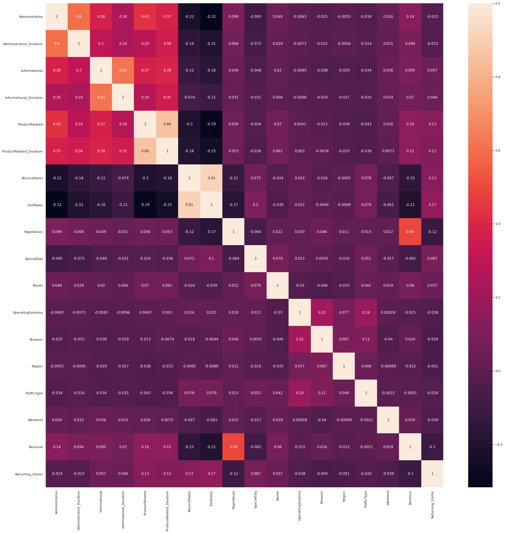
To examine which of the features are correlated with the target variable, we can run a Pearson correlation via the
Pandas corr() function. As you might have guessed, if you’re familiar with Google Analytics ecommerce data, the strongest predictor of conversion was the PageValues column, which contained the Page Value metric from GA. This is obviously higher for customers who have viewed product, basket, and checkout pages, so it makes total sense that it plays a significant role.
Similarly, customers who have viewed more product pages and spent longer looking at them were also much more likely to have purchased, as were users who shopped using specific browsers, or on certain days of the week. Although the individual correlations are low, apart from the PageValues metric, collectively these values should be enough to give our model a decent steer and have a positive impact upon performance.
df[df.columns[1:]].corr()['Revenue'][:].sort_values(ascending=False).to_frame()
| Revenue | |
|---|---|
| Revenue | 1.000000 |
| PageValues | 0.492569 |
| ProductRelated | 0.158538 |
| ProductRelated_Duration | 0.152373 |
| Informational | 0.095200 |
| Administrative_Duration | 0.093587 |
| Month | 0.080150 |
| Informational_Duration | 0.070345 |
| Weekend | 0.029295 |
| Browser | 0.023984 |
| TrafficType | -0.005113 |
| Region | -0.011595 |
| OperatingSystems | -0.014668 |
| SpecialDay | -0.082305 |
| Returning_Visitor | -0.103843 |
| BounceRates | -0.150673 |
| ExitRates | -0.207071 |
corrMatrix = df.corr()
sns.set(rc={'figure.figsize':(30, 30)})
sns.heatmap(corrMatrix, annot=True)
<AxesSubplot:>
Create the training and test data
Now we have prepared our feature set, we need to define X and y. The X feature set will include all the features we created above, minus the target variable, so we don’t give the model the answer. The y data will comprise the target variable alone.
X = df.drop(['Revenue'], axis=1)
y = df['Revenue']
We’ll now randomly split the data into a training and test dataset using the train_test_split() function. We’ll assign 30% of the data to the test group, which will be held out of training, and we’ll use the stratify option to ensure the target variable is present in equal proportions in each group. The random_state value ensures we get reproducible results each time we run the code.
X_train, X_test, y_train, y_test = train_test_split(X, y,
                                                    test_size=0.3,
                                                    random_state=0,
                                                    stratify=y
                                                   )
Create a model pipeline
Next, we’ll create a model pipeline. This will handle the encoding of our data using the ColumnTransformer()
feature, and can be used to avoid the need to manually generate some of the features we created above. This also imputes any missing values with realistic values, and scales the data before we pass it to the model.
I’ve also added some basic feature selection via SelectKBest(), and have used the Synthetic Minority Oversampling
Technique (SMOTE) to better handle class imbalance. Doing this via a function means we can easily re-use the code
elsewhere. I fiddled around with the SelectKBest parameters until I found the optimum number of features to leave in. This was around six features, which are going to be similar to those shown in the Pearson correlation above. Doing this greatly improved performance.
def get_pipeline(X, model):
    """Return a pipeline to preprocess data and bundle with a model.

    Args:
        X (object): X_train data.
        model (object): scikit-learn model object, i.e. XGBClassifier

    Returns:
        Pipeline (object): Pipeline steps.
    """

    numeric_columns = list(X.select_dtypes(exclude=['object']).columns.values.tolist())
    categorical_columns = list(X.select_dtypes(include=['object']).columns.values.tolist())
    numeric_pipeline = SimpleImputer(strategy='constant')
    categorical_pipeline = OneHotEncoder(handle_unknown='ignore')

    preprocessor = ColumnTransformer(
        transformers=[
            ('numeric', numeric_pipeline, numeric_columns),
            ('categorical', categorical_pipeline, categorical_columns),
            ], remainder='passthrough'
    )

    bundled_pipeline = imbpipeline(steps=[
        ('preprocessor', preprocessor),
        ('smote', SMOTE(random_state=1)),
        ('scaler', MinMaxScaler()),
        ('feature_selection', SelectKBest(score_func=chi2, k=6)),
        ('model', model)
    ])

    return bundled_pipeline
Select the best model
Rather than simply selecting a single model, or repeating our code manually on a range of models, we can create another function to automatically test a wide range of possible models to determine the best one for our needs. To do this we first create a dictionary containing some a selection of base classifiers, including XGBoost, Random Forest, Decision Tree, SVC, and a Multilayer Perceptron among others.
We then loop through the models, run the data through the pipeline for each one, and use cross-validation to assess the performance and reliability and validity of each model. We then store the model results in a Pandas dataframe and print the output, selecting the best one as the model with the highest ROC/AUC score.
def select_model(X, y, pipeline=None):
    """Test a range of classifiers and return their performance metrics on training data.

    Args:
        X (object): Pandas dataframe containing X_train data.
        y (object): Pandas dataframe containing y_train data.
        pipeline (object): Pipeline from get_pipeline().

    Return:
        df (object): Pandas dataframe containing model performance data.
    """

    classifiers = {}
    classifiers.update({"DummyClassifier": DummyClassifier(strategy='most_frequent')})
    classifiers.update({"XGBClassifier": XGBClassifier(verbosity=0,
                                                       use_label_encoder=False,
                                                       eval_metric='logloss',
                                                       objective='binary:logistic',
                                                      )})
    classifiers.update({"LGBMClassifier": LGBMClassifier()})
    classifiers.update({"RandomForestClassifier": RandomForestClassifier()})
    classifiers.update({"DecisionTreeClassifier": DecisionTreeClassifier()})
    classifiers.update({"ExtraTreeClassifier": ExtraTreeClassifier()})
    classifiers.update({"ExtraTreesClassifier": ExtraTreeClassifier()})
    classifiers.update({"AdaBoostClassifier": AdaBoostClassifier()})
    classifiers.update({"KNeighborsClassifier": KNeighborsClassifier()})
    classifiers.update({"RidgeClassifier": RidgeClassifier()})
    classifiers.update({"SGDClassifier": SGDClassifier()})
    classifiers.update({"BaggingClassifier": BaggingClassifier()})
    classifiers.update({"BernoulliNB": BernoulliNB()})
    classifiers.update({"SVC": SVC()})
    classifiers.update({"MLPClassifier":MLPClassifier()})
    classifiers.update({"MLPClassifier (paper)":MLPClassifier(hidden_layer_sizes=(27, 50),
                                                              max_iter=300,
                                                              activation='relu',
                                                              solver='adam',
                                                              random_state=1)})

    df_models = pd.DataFrame(columns=['model', 'run_time', 'roc_auc'])

    for key in classifiers:

        start_time = time.time()

        pipeline = get_pipeline(X_train, classifiers[key])

        cv = cross_val_score(pipeline, X, y, cv=10, scoring='roc_auc')

        row = {'model': key,
               'run_time': format(round((time.time() - start_time)/60,2)),
               'roc_auc': cv.mean(),
        }

        df_models = df_models.append(row, ignore_index=True)

    df_models = df_models.sort_values(by='roc_auc', ascending=False)
    return df_models
Running the select_model() function on our training data reveals that gradient boosting models seem to have the edge over most others, based on the base models used. The top performer was MLPClassifier(), which generated a ROC/AUC score of 0.902. We’ll select this model as our best one and examine the results in a bit more detail to see how well it works.
models = select_model(X_train, y_train)
models.head(20)
| model | run_time | roc_auc | |
|---|---|---|---|
| 14 | MLPClassifier | 0.84 | 0.901838 |
| 15 | MLPClassifier (paper) | 0.83 | 0.901241 |
| 2 | LGBMClassifier | 0.04 | 0.898587 |
| 1 | XGBClassifier | 0.05 | 0.889678 |
| 10 | SGDClassifier | 0.01 | 0.886434 |
| 13 | SVC | 0.55 | 0.885936 |
| 7 | AdaBoostClassifier | 0.06 | 0.884092 |
| 3 | RandomForestClassifier | 0.19 | 0.878788 |
| 11 | BaggingClassifier | 0.04 | 0.856906 |
| 12 | BernoulliNB | 0.01 | 0.851748 |
| 9 | RidgeClassifier | 0.01 | 0.849696 |
| 8 | KNeighborsClassifier | 0.01 | 0.836910 |
| 5 | ExtraTreeClassifier | 0.01 | 0.750767 |
| 6 | ExtraTreesClassifier | 0.01 | 0.749719 |
| 4 | DecisionTreeClassifier | 0.01 | 0.717740 |
| 0 | DummyClassifier | 0.01 | 0.500000 |
Examine the performance of the best model
By re-running the get_pipeline() function on our selected mode, the MLPClassifier(), we can generate predictions and assess their accuracy on the test data. What this shows is that the MLPClassifier model generated a ROC/AUC score of 0.902 on the training data, which is really good, but a slightly lower ROC/AUC score of 0.836 on the test data, with an overall accuracy of 0.88.
selected_model = MLPClassifier()
bundled_pipeline = get_pipeline(X_train, selected_model)
bundled_pipeline.fit(X_train, y_train)
y_pred = bundled_pipeline.predict(X_test)
roc_auc = roc_auc_score(y_test, y_pred)
accuracy = accuracy_score(y_test, y_pred)
f1_score = f1_score(y_test, y_pred)
Testing various models reveals similar results. Although the scores themselves aren’t bad, and similar papers have generated similar results, the distance between these scores is a sign that our model is overfitting a bit, so we’ve still got some room for improvement.
The F1 score at 0.667 is OK, but would benefit from being improved. The paper provides some insight into how this was done. I’m going to skip this step for brevity. The results are OK, but in a real world situation, you’d spend much more time tweaking the model to improve the outputs.
print('ROC/AUC:', roc_auc)
print('Accuracy:', accuracy)
print('F1 score:', f1_score)
ROC/AUC: 0.8366354623949763
Accuracy: 0.8807785888077859
F1 score: 0.6671698113207547
print(classification_report(y_test, y_pred))
              precision    recall  f1-score   support

           0       0.96      0.90      0.93      3127
           1       0.59      0.77      0.67       572

    accuracy                           0.88      3699
   macro avg       0.77      0.84      0.80      3699
weighted avg       0.90      0.88      0.89      3699
Examining the confusion matrix for the selected model, which we’ve not even tuned yet, shows that we correctly predicted that 2816 out of 3127 customers (90%) wouldn’t purchase during their session, and we correctly predicted that 77% of customers who would purchase during their sessions.
Clearly, there’s still more we could do, and my quick-and-dirty results aren’t as good as those of the authors, but it’s not a bad start, and the overall accuracy of 88% is not too shabby. The results show that it’s possible to predict purchase intention from consumer behaviour data with a good degree of accuracy.
confusion_matrix(y_test, y_pred, labels=np.unique(y_test))
array([[2816,  311],
       [ 130,  442]])
Using the model’s predictions
According to the Sakar et al paper, the goal was to develop a model that would increase the sales volumes of the online shopping retailer by 20% by automatically serving promotions to customers the model identified had high shopping intention but were likely to abandon. This was achieved by setting a “trigger threshold” based on their probability of conversion. Using this prediction, the retailer can then “take timely actions accordingly to improve the shopping cart abandonment and purchase conversion rates.”
They say that “If the value of ‘ProductRelated’ or ‘ProductRelated_Duration’ is on the high side, it can represent that customers are interested in our products, or they are hesitating. At this moment, we can encourage the customers to make the orders by sending additional advertisements or discounts automatically.
“Through the ‘Month’ data, we can see that the sales rate is totally different from the slack season and peak season. So, our company can launch promotional activities to increase the sales rate in the slack season.”
Further reading
- Baati, K. and Mohsil, M., 2020, June. Real-Time Prediction of Online Shoppers’ Purchasing Intention Using Random Forest. In IFIP International Conference on Artificial Intelligence Applications and Innovations (pp. 43-51). Springer, Cham.
- Kabir, M.R., Ashraf, F.B. and Ajwad, R., 2019, December. Analysis of Different Predicting Model for Online Shoppers’ Purchase Intention from Empirical Data. In 2019 22nd International Conference on Computer and Information Technology (ICCIT) (pp. 1-6). IEEE.
- Sakar, C.O., Polat, S.O., Katircioglu, M. and Kastro, Y., 2019. Real-time prediction of online shoppers’ purchasing intention using multilayer perceptron and LSTM recurrent neural networks. Neural Computing and Applications, 31(10), pp.6893-6908.
Matt Clarke, Saturday, May 29, 2021


Other posts you might like

How to tune a LightGBMClassifier model with Optuna
The LightGBM model is a gradient boosting framework that uses tree-based learning algorithms, much like the popular XGBoost model. LightGBM supports both classification and regression tasks, and is known for...

How to create a customer retention model with XGBoost
Although all business know the importance of retaining customers, few companies are actually able to measure customer retention accurately, and fewer still can predict which ones will churn or be...
